Scan Detection: A Data Mining Approach - MINDS - Minnesota ...

Scan Detection: A Data Mining Approach Gy¨orgy J. Simon

Hui Xiong

Eric Eilertson

Vipin Kumar

Computer Science Univ. of Minnesota [email protected]

MSIS Dept. Rutgers Univ. [email protected]

Computer Science Univ. of Minnesota [email protected]

Computer Science Univ. of Minnesota [email protected]

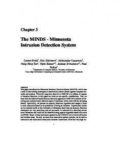
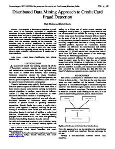
Abstract A precursor to many attacks on networks is often a reconnaissance operation, more commonly referred to as a scan. Despite the vast amount of attention focused on methods for scan detection, the state-ofthe-art methods suffer from high rate of false alarms and low rate of scan detection. In this paper, we formalize the problem of scan detection as a data mining problem. We show how the network traffic data sets can be converted into a data set that is appropriate for running off-the-shelf classifiers on. Our method successfully demonstrates that data mining models can encapsulate expert knowledge to create an adaptable algorithm that can substantially outperform state-ofthe-art methods for scan detection in both coverage and precision. 1

Introduction

A precursor to many attacks on networks is often a reconnaissance operation, more commonly referred to as a scan. Identifying what attackers are scanning for can alert a system administrator or security analyst to what services or types of computers are being targeted. Knowing what services are being targeted before an attack allows an administrator to take preventative measures to protect the resources e.g. installing patches, firewalling services from the outside, or removing services on machines which do not need to be running them. Given its importance, the problem of scan detection has been given a lot of attention by a large number of researchers in the network security community. Initial solutions simply counted the number of destination IPs that a source IP made connection attempts to on each destination port and declared every source IP a scanner whose count exceeded a threshold [16]. Many enhancements have been proposed [18, 5, 15, 9, 14, 13], but despite the vast amount of expert knowledge spent on these methods, current, state-of-the-art solutions still suffer from high percentage of false alarms or low ratio of scan detection.

For example, a recently developed scheme by Jung [5] has better performance than earlier methods, but it requires that scanners attempt connections to several hosts on a destination port before they can be detected. This constraint limits the scheme’s applicability because a sizable portion of the scanners attempt connections to only one host on each port in a typical observation window giving a net result of poor coverage. Data mining techniques have been successfully applied to the generic network intrusion detection problem[8, 2, 10], but not to scan detection.1 In this paper, we present a method for transforming network traffic data into a feature space that successfully encodes the accumulated expert knowledge. We show that an off-the-shelf classifier, Ripper[3], can achieve outstanding performance both in terms of missing only very few scanners and also in terms of very low false alarm rate. While the rules generated by Ripper make perfect sense from the domain perspective, it would be very difficult for a human analyst to invent them from scratch. 1.1 Contributions This paper has the following key contributions: • We formalize the problem of scan detection as a data mining problem and present a method for transforming network traffic data into a data set that classifiers are directly applicable to. Specifically, we formulate a set of features that encode expert knowledge relevant to scan detection. • We construct carefully labeled data sets to be used for training and test from real network traffic data at the University of Minnesota and demonstrate that Ripper can build a high-quality predictive model for scan detection. We show that our method is capable of very early detection (as early as 1 Scans were part of the set of attacks used in the KDD Cup ’99 [1] data set generated from the DARPA ’98/’99 data sets. Nearly all of these scans were of the obvious kind that could be detected by the simplest threshold-based schemes that simply look at the number of hosts touched in a period of time or connection window.

the first connection attempt on the specific port) without significantly compromising the precision of the detection. • We present extensive experiments on real-world network traffic data. The results show that the proposed method has substantially better performance than the state-of-the-art methods both in terms of coverage and precision. 2 Background and Related Works Until recently, scan detection has been thought of as the process of counting the distinct destination IPs talked to by each source on a given port in a certain time window [16]. This approach is straightforward to evade by decreasing the frequency of scanning. With a sufficiently low threshold (to allow capturing slow scanners), the false alarm rate can become high enough to render the algorithm useless. On the other hand, higher thresholds can leave slow and stealthy scanners undetected. A number of more sophisticated methods [9, 18, 15, 5, 4] have been developed to address the limitations of the basic method. Robertson [15] assigns an anomaly score to a source IP based on the number of failed connection attempts it has made. This scheme is more accurate than the ones that simply count all connections since scanners tend to make failed connections more frequently. However, the scanning results still vary greatly depending on the definition of a failed connection and how the threshold is set. Lickie [9] uses a statistical approach to determine the likelihood of a connection being normal versus being part of a scan. The main flaw of this algorithm is that it generates too many false alarms when access probabilities are highly skewed (which is often the case.) SPICE [18] is another statistical-anomaly based system which sums the negative log-likelihood of destination IP/port pairs until it reaches a given threshold. One of the main problems with this approach is that it will declare a connection to be a scan simply because it is to a destination that is infrequently accessed. The intuition behind SPICE is partly correct. It is true that destinations that are accessed only by scanners are rare, but the converse is not true. A scheme proposed by Ert¨oz et al. [4] assigns a scan score to each source IP on each destination. If the requested service is offered – regardless of how infrequently it is used – the score is not increased. If the requested service does not exist, the score is increased by the reciprocal of the log frequency of the destination. This scheme achieves fairly good performance, and is generally comparable to the TRW scheme in precision and recall that we describe next.

The current state-of-the-art for scan detection is Threshold Random Walk (TRW) proposed by Jung et al. [5]. It traces the source’s connection history performing sequential hypothesis testing. The hypothesis testing is continued until enough evidence is gathered to declare the source either scanner or normal. Assuming that the source touched k distinct hosts, the test statistics (the likelihood ratio of the source being scanner or normal) is computed as follows:  if the first connection to k  γ0 Y host i fails Λ=  1 otherwise, i=1 γ1

where γ0 and γ1 are constants. The source is declared a scanner, if Λ is greater than an upper threshold; normal, if Λ is less than a lower threshold. The thresholds are computed from the nominal significance level of the tests. It is worth pointing out that in a logarithmic space, when log γ0 = 1, then log Λ is increased by one every time a first connection fails and is decreased by one every time a first connection succeeds. The threshold in this logarithmic space (the log of the threshold in the original space) is number of consecutive first-connection failures required for a source to be declared a scanner. For simplicity, in the rest of the paper, when we say threshold, we will refer to the log-threshold. The authors of TRW recommend using a threshold of 4 (that is TRW is going to declared an IP scanner only after having made at least 4 observations). At this threshold, TRW can achieve high precision. Reducing the threshold to 1 will result in an unacceptably high rate of false alarms rendering TRW unable to reliably detect scans that only make one connection attempt within the observation period. These false alarms are primarily caused by P2P and backscatter traffic. In recent years when the legality of certain uses of file sharing networks (based on P2P) has been questioned in the courtrooms, P2P networks started increasingly utilizing random ports to avoid detection. Peers agree upon a (practically) randomly chosen destination port that they conduct their communications on. They also maintain a list of the pairs of their peers. Upon trying to re-connect to a P2P network, the host makes connection attempts to the hosts on its list of peers. The hosts on the list may not offer the service any more – e.g. they may be turned off or their dynamic IP address changed. To a scan detector, a P2P host unsuccessfully trying to to connect to its peers may appear as a scan [7, 6]. Backscatter traffic is another type of network traffic that can be easily mistaken for scan. Backscatter

traffic typically originates from a server under denialof-service (DoS) attack. In the course of a DoS attack, attackers send a server (the victim) such a large amount of network packets that the server becomes unable to render its usual service to its legitimate clients. The attackers also falsify the source IP and source port fields in these packets, so when the server responds,it sends its replies to the falsified (random) addresses. For a sufficiently large network, there can be enough falsified addresses that fall within the network space, such that replies from the victim will make it seem like a scanner: the victim is unsolicitedly sending packets to hosts that may not even exist [11]. 3

Definitions and Method Description

In the course of scanning, the attacker aims to map the services offered by the target network. There are two general types of scans (1) horizontal scans, where the attacker has an exploit at his disposal and aims to find hosts that are exploitable by checking many hosts for a small set of services; and (2) vertical scan, where the attacker is interested in compromising a specific computer or a small set of specific computers. They often scan for dozens or hundreds of services. Source IP, destination port pairs (SIDPs) are the basic units of scan detection; they are the potential scanners. Assume that a user is browsing the Web (destination port 80) from a computer with a source IP S. Further assume that S is infected and is simultaneously scanning for port 445. Our definition of a scanner allows us to correctly distinguish between the user surfing the Web (whose SIDP < S, 80 > is not a scanner) from the SIDP < S, 445 > which is scanning. Scan Detection Problem Given a set of network traffic records (network traces) each containing the following information about a session (source IP, source port, destination IP, destination port, protocol, number of bytes and packets exchanged and whether the destination port was blocked), scan detection is a classification problem in which each SIDP, whose source IP is outside the network being observed, is labeled as scanner if it was found scanning or non-scanner otherwise. Overview of the Solution The essence of our proposed method is the assumption that given a properly labeled training data set and the right set of features, data mining methods can be used to build a predictive model to classify SIDPs (as scanner or non-scanner). In case of the scan detection problem, we will observe SIDPs over as long a time period as our computational resources allow and label them with high preci-

sion2 . We will train a classifier – any off-the-shelf classifier – on this precisely labeled data and let the classifier learn the patterns characteristic of scanning behavior. Then we can apply this classifier to unlabeled data collected over a much shorter observation period and (as we will demonstrate later) successfully detect scanners. The success of this method depends on (1) whether we can label the data accurately and (2) whether we have derived the right set of features that facilitate the extraction of knowledge. Section 3.1 and 3.2 will elaborate on these points. Choice of classifier. Although most classifiers are applicable to our problem, some classifiers are better suited than others. Our understanding of data mining classifier algorithms guided us towards choosing Ripper. We chose Ripper, because (a) the data is not linearly separable, (b) most of the attributes are continuous, (c) the data has multiple modes and (d) the data has unbalanced class distribution. Ripper can handle all of these properties quite well. Furthermore, it produces a relatively easily interpretable model in the form of rules allowing us to assess whether the model reflects reality well or if it is merely coincidental. An additional benefit is that classification is computationally inexpensive 3 . The drawback of Ripper is its greedy optimization algorithm and its tendency to overfit the training data at times. These drawbacks did not set us back too much; we encountered the overfit problem with visible effect only on one occasion. 3.1 Features The key challenge in designing a data mining method for a concrete application is the necessity to integrate the expert knowledge into the method. A part of the knowledge integration is the derivation of the appropriate features. Table 1 provides the list of features that we derived. The first set of features (srcip, scrport, dstport) serve to identify a record; these features are not used for classification. The second set of features contains statistics about the destination IPs and ports. These features provide an overall picture of the services and hosts involved in the source IP’s communication patterns. The first feature in this group, ndstips, is the revered heuristic that defined early scan detection schemes. In addition, we provide features to show whether the source IP was using a few 2 As we will explain in Section 3.2, despite our claims about the poor performance of the current scan detection schemes, labeling at a very high precision is possible under certain circumstances. 3 Building the model is computationally expensive, but it can be performed off-line. It is the actual classification that needs to be carried out in real-time.

Table 1: The List of Features Extracted from the Network Trace Data Feature srcip srcport dstport

Description Source IP Source port or 0 for multiple source ports Destination port Destination IP and Port Statistics ndstip Number of distinct destination IPs touched by the source IP ndstports Number of distinct destination ports touched by the source IP avgdstips Number of distinct destination IPs averaged over all destination ports touched by the source IP. maxdstips Maximum number of distinct destination IPs over all destination ports that the source IP touched. Statistics Aggregated over All Destination Ports server The ratio of (distinct) destination IPs that provided the service that the source IP requested. client The ratio of (distinct) destination IPs that requested service from the source IP on the destination port during the 24 hours preceding the experiment time. nosrv The ratio of (distinct) destination IPs touched by the source IP that offered no service on dstport to any source during the observation period. dark The ratio of (distinct) destination IPs that has been inactive for at least 4 weeks prior to the experiment date. blk The ratio of (distinct) destination IPs that were attempted connections to by the source IP on a blocked port during the experiment. p2p The ratio of (distinct) destination IPs that have actively participated in P2P traffic over the 3 weeks prior to the test date. Statistics on Individual Destination Ports i ndstips ) i none Same definitions as above except i dark measured on a single dstport. i blk

services on many hosts, or many services on a few hosts (avgdstips, maxdstips). The third set of features have two goals. First, they help determine the role of the source IP: high values of client (percentage of inside IPs that are clients of the source IP) and low values of server (percentage of inside IPs that offer service to the source IP) indicate that the source IP is a server, otherwise it is a client. The remaining features nosrv, dark, blk, p2p allow us to assess the source IP’s behavior.

The fourth set of features describe the role and behavior of the source IP on a specific destination port. The individual features serve the same purpose as their siblings in the third set. The importance of including the fourth group lies in the observation that certain source IPs exhibit vastly different behavior on some ports than on the majority of the ports they touch. An example could be a P2P host which is infected by a worm: the host is engaged in its usual P2P activity on a number of ports and it is also scanning on some ports. 3.2 Labeling the Data Set The goal of labeling is to assign each < source IP, destination port > pair (SIDP) a label that describes its behavior best. We distinguish between the following broad behavior classes (1) scanning (labeled as SCAN ), (2) traditional client/server applications (NRML), (3) P2P (P2P ) and (4) Internet noise (NOISE ) [12]. While general scan detection schemes have been criticized for their high false alarm rates or low coverages, we claim that we are able to reliably label a set of SIDPs that appear within a short time window by observing their behavior over a long period. This is possible because our labeling scheme is different from earlier scan detection methods in the following key respects. The most crucial difference lies in the length of the observation period. The sharp-eyed Readers may have noticed that some of the features in Table 1 include information about inactive IPs and P2P hosts. Automatically constructing an accurate list of inactive IPs or P2P hosts requires very long observations. We use 22 days of traffic data (95 GB of compressed netflow data) to construct these lists. Fortunately, the changes to these lists are marginal and hence they can be continuously updated during normal operation. In sharp contrast to the above lists, features in Table 1 are so dynamic that under the performance constraints of production use (real-time classification), we can only maintain information within a 20-minute window: scan detection must be done based on 20 minutes of observation. On the other hand, the labeling of the training set can be performed off-line. Upon training, we select a 20-minute window and observe the source IPs that were active in that 20-minute window for 3 days. The extra observations we obtained by watching the IPs for 3 days enables us to label them at considerably higher confidence. Even existing schemes are capable of scan detection at high precision – at high thresholds. High thresholds require more observations, causing the coverage to become intolerably small. By drastically increasing the time window (from 20 minutes to 3 days), we provide

additional observations that helps increase the coverage. Second, existing scan detection methods observe the behavior of the source IPs on specific ports separately. In our labeling scheme, on top of examining the activities of a source IP on each individual destination port separately, we also correlate their activities across ports. Certain types of traffic, most prominently P2P and backscatter, can only be recognized when information is correlated across destination ports. Third, practical scan detection schemes have requirements such as being able to run in real-time. As we have discussed before, training (labeling the training data and building the data mining model) can be performed off-line. This allows us to perform more expensive computations including tracing the connection history of source IPs for 3 days instead of 20 minutes. For the details of the labeler, the Reader is referred to [17]. 4

Evaluation

4.1 Description of the Data Set For our experiments, we used real-world network trace data collected at the University of Minnesota between the 1st and the 22nd March, 2005. The University of Minnesota network consists of 5 class-B networks with many autonomous subnetworks. Most of the IP space is allocated, but many subnetworks have inactive IPs. We collected information about inactive IPs and P2P hosts over 22 days and we used 03/21/2005 and 03/22/2005 for the experiments. To test generalizability (in other words to reduce possible dependence on a certain time of the day), we took samples every 3 hours and performed our experiments on each sample. As far as the length of each observation period (sample) is concerned, longer observations result in better performance but delayed detection of scans. Therefore, in production use, the scan detector will operate in a streaming mode, where the periods of observation will vary in length across SIDPs: lengths will be kept to the minimal amount sufficient for conclusive classification of each SIDP. Now, the system works in batch mode, so we keep as many observations as possible. Our memory (1 GB) allows us to store and process 4 million flows, which approximately corresponds to 20 minutes of traffic. Table 2 describes the traffic in terms of number of (SIDP) combinations pertaining to scanning-, P2P- and normal traffic and Internet noise. The proportion of normal traffic appears small. This has two reasons: (a) arguably the dominant traffic of today’s Internet is P2P [7] and (b) even though P2P is also “normal” traffic, according to our definition,

Table 2: The distribution of (source IP, destination ports) (SIDPs) over the various traffic types for each traffic sample ID 01 02 03 04 05 06 07 08 09 10 11 12 13

Day.Time 0321.0000 0321.0300 0321.0600 0321.0900 0321.1200 0321.1500 0321.1800 0321.2100 0322.0000 0322.0300 0322.0600 0322.0900 0322.1200

Total 67522 53333 56242 78713 93557 85343 92284 82941 69894 63621 60703 78608 91741

scan 3984 5112 5263 5126 4473 3884 4723 4273 4480 4953 5629 4968 4130

p2p 28911 19442 19485 32573 38980 36358 39738 39372 33077 26859 25436 33783 43473

normal 6971 9190 8357 10590 12354 10191 10488 8816 5848 4885 4467 7520 6319

noise 4431 1544 2521 5115 4053 5383 5876 1074 1371 4993 3241 4535 4187

dnknw 23225 18045 20616 25309 33697 29527 31459 29406 25118 21931 21930 27802 33632

the normal behavior class consists of the traditional client/server type traffic which excludes P2P. Other than the distribution of the SIDPs over the different behavior classes, the traffic distribution is as expected. The proportion of normal traffic is highest during business hours, P2P – for the largest part attributed to students living in the residential halls – peaks late afternoon and during the evening, and scans are most frequent in the early morning hours. The number of “don’t know”s, that is traffic with insufficient observation, seems to be more correlated with normal and P2P traffic than with scanning traffic. The patterns repeat during the next day. Evaluation Measures The performance of a classifier is measured in terms of precision, recall and Fmeasure. For a contingency table of

actual Scanner actual not Scanner

prec

=

recall

=

Fm

=

classified as Scanner TP FP

classified as not Scanner FN TN

TP TP + FP TP TP + FN 2 ∗ prec ∗ recall . prec + recall

Less formally, precision measures the percentage of scanning (source IP, destination port)-pairs (SIDPs) among the SIDPs that got declared scanners; recall measures the percentage of the actual scanners that were discovered; F-measure balances between precision and recall.

4.2 Comparison to the State-of-the-Art To obtain a high-level view of the performance of our scheme, we built a model on the 0321.0000 data set (ID 1) and tested it on the remaining 12 data sets. The performance results were compared to that of Threshold Random Walk (TRW), which is considered to be the stateof-the-art. Figure 1 depicts the performance of our proposed scheme and that of TRW on the same data sets.

Performance of Ripper 1 0.8 0.6 0.4 Precision

Performance Comparison 1

0.2

0.8

0

Recall F−measure 3

5

7 9 Test Set ID

11

13

0.6

Figure 2: The performance of the proposed scheme on the 13 data sets in terms of precision (topmost line), F-measure (middle line) and recall (bottom line). The model was built on data set ID 1.

0.4

0.2

0

Prec

Rec F−m Ripper

Prec

Rec TRW

F−m

Figure 1: Performance comparison between the proposed scheme and TRW. From left to right, the six box plots correspond to the precision, recall and F-measure of our proposed scheme and the precision, recall and F-measure of TRW. Each box plot has three lines corresponding (from top downwards) to the upper quartile, median and lower quartile of the performance values obtained over the 13 data sets. The whiskers depict the best and worst performance. One can see that not only does our proposed scheme outperform the competing algorithm by a wide margin, it is also more stable: the performance varies less from data set to data set (the boxes on Figure 1 appear much smaller). Figure 2 shows the actual values of precision, recall and F-measure for the different data sets. The performance in terms of F-measure is consistently above 90% with very high precision, which is important, because high false alarm rates can rapidly deteriorate the usability of a system. The only jitter occurs on data set # 7 and it was caused by a single source IP that scanned a single destination host on 614(!) different destination ports meanwhile touching only 4 blocked ports. Not only is such behavior uncharacteristic of our network (the only other vertical scanner we saw was the result of a ’ScanMyComputer’ service touching as many blocked ports as expected), but it is more characteristic of P2P traffic causing the misclassification of this scanner.

As discussed earlier, the authors of TRW recommend a threshold of 4. In our experiments, we found, that TRW can achieve better performance (in terms of F-measure) when we set the threshold to 2, this is the threshold that was used in Figure 1, too. In Figure 3, we examine how the TRW’s performance depends on the threshold. The five box plots represent the performance at the five thresholds between 1 and 5. The horizontal lines of the boxes correspond to the upper quartile, median and lower quartile of the 13 performance measurements (one for each of the 13 data sets) and whiskers extend out to the extreme performance values. Figure 3 shows that the threshold balances between precision and recall. At low thresholds (such as 1), TRW achieves high recall by declaring anything a scanner that makes one failed connection more than successful connections. As a consequence, a lot of false alarms are generated, typically caused by P2P and backscatter. The other extreme is the high threshold of 5, where only the most obvious scanners are caught. P2P and backscatter are not declared scanners at such high thresholds, because the chances of them making connection attempts to 5 distinct destination IPs on the same random destination port are slim. In the followings we show that the success of the data mining approach stems from its ability to correlate the behavior of a source IP on multiple hosts. This allows both early detection and accurate categorization of scanning-like non-scanning traffic. To illustrate the benefits of data mining and to explain the above results, let us consider the concrete ex-

Performance of TRW (Precision)

Performance of TRW (Recall)

Performance of TRW (F−measure)

1

1

1

0.8

0.8

0.8

0.6

0.6

0.6

0.4

0.4

0.4

0.2

0.2

0.2

0

1

2

3 Treshold

4

5

0

1

2

3 Treshold

4

0

5

1

2

3 Treshold

4

5

Figure 3: Box plots of the precision (left), recall (middle) and F-measure (right) of TRW at five different thresholds (horizontal axis). ample of the data set 0321:1200, where our proposed approach achieved close to median of the 13 performance values. Claim 1. The correlation of evidence across destination ports allows the data mining approach to detect scanners earlier, in some cases as early as the first connection attempt on a destination port (provided that the same source IP previously made connection attempts to other ports). Intuitively, this claim is true, since positive evidences from different data sources can certainly increase the confidence in our decisions. This is widely recognized as joint learning. In order to experimentally demonstrate our claim, we look at a portion of the traffic that made connection attempts to no more than one destination IP on any destination port within the 20-minute window. Out of the 93,557 SIDPs, 66,872 satisfy this condition, which is a very large portion of the traffic. Out of the 66,872 SIDPs, we were unable to label 29,397. The SIDPs that we were able to label have the following distribution: SCAN 3,014

P2P 28,078

NRML 5,995

NOISE 388

Total 37,475

In Table 3, we present the results of our proposed scheme and that of TRW at a threshold of 1. Since no SIDP made connection attempts to two distinct destination IPs on the same port, TRW at higher thresholds would not find scanners. The results show that TRW1 found more scanners, but its false alarm rate was unacceptably high. Most of the false alarms are due to P2P and Internet noise. For completeness, in Table 4 we show the number of SIDPs that we were unable to label but got declared scanners by the two schemes.

Table 3: The performance of the data mining approach and some competing schemes on the portion of the data set that contains source IPs that never made connection attempts to more than 1 destination IP on a single destination port. ’TP’ denotes the number of SIDPs classified correctly as scanner, ’FN’ the scanning SIDPs that did not get identified and ’FP’ the SIDPs that were predicted to scan but they did not. Scheme TP FN FP Prec Rec Fm TRW1 2908 106 23760 0.1090 0.9648 0.1959 Ripper 2630 384 54 0.9799 0.8726 0.9231

Table 4:

The number of SIDPs whose true nature is unknown classified as scanner by the different schemes Scheme Unlabeled Classified as Scanner

TRW1

Ripper

17,407

1,144

Although not directly relevant to proving Claim 1, in order to present the Reader with a full set of results, in Table 5, we show the performance of the above schemes on the complementary data set, namely the portion of the data set that contains the SIDPs that made connection attempts to at least two distinct destination IPs on at least one port. There are 26,685 SIDPs satisfying this condition, out of which we managed to label 22,385. The distribution of traffic classes over these 22,385 SIDPs is as follows. SCAN 1,459

P2P 10,902

NRML 6,359

NOISE 3,665

Total 22,385

Since it can be advantageous for TRW to use higher thresholds on this portion of the data, we present results for TRWk, where the threshold is k, k = 1, . . . , 5. TRW exhibits the behavior described earlier: higher thresholds result in increasing precisions but rapidly

Table 5: The performance of the data mining approach and

Table 7: Performance Comparison on Internet Noise and

the competing schemes on the complementary (to Table 3) portion of the data set. Scheme TP FN FP Prec Rec Fm TRW1 1389 70 8952 0.1343 0.9520 0.2354 155 1760 0.4256 0.8938 0.5766 TRW2 1304 TRW3 645 814 261 0.7119 0.4421 0.5455 TRW4 485 974 45 0.9151 0.3324 0.4877 TRW5 447 1012 18 0.9613 0.3064 0.4647 Ripper 1406 53 23 0.9839 0.9637 0.9737

Scanning Traffic. Scheme TP TRW-1 1562 TRW-2 118 538 TRW-P Simple 219 Simple-P 184 Ripper 2549

deteriorating coverage. In terms of F-measure, it achieved its peak performance at a threshold of 2, but still falling behind Ripper by a wide margin. Claim 2. Through correlating evidence across destination ports, the data mining approach is capable of filtering out scanning-like non-scanning traffic types such as P2P or backscatter. Certain types of traffic, including P2P and Internet noise – most prominently backscatter – apart from some obvious cases (touching only P2P hosts on a certain ports) can only be recognized by observing the behavior of the source IP across ports. Table 6 presents the performance of the data mining based scheme and some competing schemes on P2P and scanning traffic only. We are using the same model (built on the first data set, 0321:1200) as in case of Claim 1. We continue using the same test set (0321.1200), but we removed all instances that are not scanners or P2P. There are 38,980 P2P and 4,473 scanning SIDP’s in this portion of the test set. The competing schemes are TRW at a threshold of 1 (TRW-1), TRW at a threshold of 2 (TRW-2) and TRW-P, which is basically the TRW-1 scheme but we applied a simple P2P filtering: any source IP that makes connection attempts to a P2P hosts is not considered a scanner on that destination port. Table 6: Performance Comparison on P2P and Scanning Traffic. Scheme TRW-1 TRW-2 TRW-P Ripper

TP 1715 137 594 2878

FN 1519 3097 2640 356

FP 16414 1039 6774 62

Prec 0.0946 0.1165 0.0806 0.9789

Rec 0.5303 0.0424 0.1837 0.8899

Fm 0.1606 0.0621 0.1121 0.9323

We evaluated the same set of schemes on backscatter traffic, too. We use the same model and the same test set (0321:1200), but this time we removed all instances that were not noise or scanners from the original test set. There are 4,473 scanner and 4,053 noise SIDPs left. Table 7 presents the results.

FN 1323 2767 2347 2666 2701 336

FP 2325 163 747 452 404 0

Prec 0.4019 0.4199 0.4187 0.3264 0.3129 1.0000

Rec 0.5414 0.0409 0.1865 0.0759 0.0638 0.8835

Fm 0.4613 0.0745 0.2580 0.1232 0.1060 0.9382

The results for P2P and backscatter are similar. While our proposed scheme’s performance is characterized by very high precision, high recall, it is evident that without recognizing P2P, high performance is unattainable. This comparison was not exactly fair, since in the original paper, TRW does not have P2P information at its disposal. However our experiments on the TRW-P scheme show, that even when information about P2P is available, it is not straightforward how one can use it. One needs to correlate ports in order to successfully distinguish P2P from scanners. Claim 3. The data mining approach was capable of extracting the characteristics of scanning behavior from the long (3-day) observation and it was subsequently capable of applying this knowledge to successfully classify data from short (20-minute) observation. Table 8 depicts the rules generated by Ripper on 0321:000. In general, the rules make sense. In fact, Rule #2, which is responsible for the lion’s share of the work is essentially an enhanced version of TRW’s heuristic (of failed vs. successful first connections). Similarly to TRW, Rule #2 also takes failure (and success) into account but it goes further by correlating this knowledge across ports. It does not stop there, it also correlates it with other evidence, the usage of blocked ports. Rule #1 did not get invoked at all possibly indicating to the Reader that it may not be as useful in practice. Nevertheless, Rule #1 does makes sense, too. It did not get invoked simply because it is geared towards blocked scanners – SIDPs who scan multiple hosts on multiple ports. This test data set contained no such scanners; our scanners (in this data set) either scanned vertically (with half of the ports blocked) or horizontally, where less than half of the connection attempts were blocked (but may have touched inactive IPs). The former scanners were caught in large by Rule #2 and the horizontal scanners were caught by the rest of the rules. From the ndstips>=2 and ndstports= 0.5 nosrv >= 0.6667 indstips >= 2 More than half of the destination IPs touched were touched on blocked destination ports, mostly service was not offered and the source IP touched at least 2 distinct IPs on the current destination port. 2

3764

blk >= 0.5 nosrv >= 0.7778 More then half of the IPs were touched on blocked destination ports and service is almost never offered.

3

35

iblk >= 1 ndstips >= 2 ndstports = 1 pp = 0.5476 . iblk >= 1 nosrv >= 1 blk >= 0.5 . blk >= 0.3333 nosrv >= 0.8889 . blk >= 0.5 nosrv >= 1 . blk >= 0.4 nosrv >= 0.75 . blk >= 0.3333 nosrv >= 0.5 iblk >= 1 . blk >= 0.3333 nosrv >= 0.5714 . blk >= 0.3333 nosrv >= 0.875 .

4.2.1 Variations to Rule #2 As mentioned before, Rule #2 has the largest contribution to the high performance of our proposed scheme. Since this rule is so dominant, yet appears very generic, it is reasonable to assume that models built on other data sets contain similar rules. Indeed, examination of the models built on the other 12 data sets revealed that 8 other data sets have close variants of Rule #2. Table 9 shows these rules. The fact that the rule appears with a wide range

of thresholds (blk varying between .3 and .5 and nosrv varying between .54 and 1) reassures us that the rule is indeed generic. Figure 4 depicts the performance of Ripper (in terms of F-measure) on the test set 0321.1200 for nosrv and blk thresholds varying between 0 and 100 %. Fmeasure values less than .85 were encountered only when nosrv or blk was 0. To enhance visibility, we replaced all values (101 values) less than .85 with .85. The results show that the dependence of the performance upon a correctly chosen threshold is minimal. For blk, the performance is practically constant as long as blk≥ 50% (and experiences a maximum of 2% drop according to F-measure and precision for blk>1%); for nosrv, it performs best between 1% and 85%. These results are not surprising. In [5], Jung has pointed out that network traffic has a bimodal distribution in terms of the ratio of < destination IP, port> pairs offering the requested service: either almost all of them or almost none of destinations offered the requested service. As far as the blk feature is concerned, there is a logical explanation for its characteristics. There are N = 216 ports, out of which B are blocked. If a source IP randomly selects a set of n ports, then the number b of blocked port in the set follows Binomial(n, B/N ). Since B