scheduled runs, while satisfying the constraint that the number of boarding .... Line carriers are characterized by a vehicle capacity Qâââ++, and by an alighting ...
SCHEDULE-BASED TRANSIT ASSIGNMENT: A NEW DYNAMIC EQUILIBRIUM MODEL WITH VEHICLE CAPACITY CONSTRAINTS
Natale Papola, Francesco Filippi, Guido Gentile, Lorenzo Meschini Dipartimento di Idraulica Trasporti e Strade, Università degli Studi di Roma “La Sapienza”
ABSTRACT We propose in this paper a new approach for modelling congested transit networks with fixed timetables where it may happen that there is not enough room onboard to allow all users waiting for a given line on the arriving carrier, so that passengers need to queue at the stop until the service becomes actually available to them. The traditional approach to reproduce this phenomenon within the established framework of diachronic graphs, where the supply is represented through a space-time network, is to introduce volume-delay functions for waiting arcs, which are meant to discourage passengers from boarding overcrowded carriers. However, this produces a distortion on the cost pattern, since passengers who achieve boarding do not suffer any additional cost, and may also cause numerical instability. To overcome these limitations we extend to the case of scheduled services an existing Dynamic Traffic Assignment model, allowing for explicit capacity constraints and FIFO queue representation, where the equilibrium is formulated as a fixed point problem in terms of flow temporal profiles. The proposed model propagates time-continuous flows of passengers on the pedestrian network and time-discrete point-packets of passengers on the line network. To this end, the waiting time pattern, corresponding to a given flow temporal profile of pedestrians who reach a stop to ride a certain line,
2
Natale Papola, Francesco Filippi, Guido Gentile, Lorenzo Meschini
has a saw-tooth temporal profile such to concentrate passengers on the scheduled runs, while satisfying the constraint that the number of boarding users must not be higher than the onboard residual capacities. An MSA algorithm is also devised, whose efficiency is tested on the regional transit network of Rome.
1
INTRODUCTION
The pricing and rationing measures applied to discourage the use of private cars, in order to alleviate the increasing road congestion and the consequent worsening pollution, are not always coupled with a consistent policy aimed at improving the performances, or at least the capacity, of the transit system. As a result, in many modern cities the problem of full transit carriers is becoming more and more relevant, both for the urban system and for the regional system used by commuters. Although this situation should be avoided through a correct design of the transit network by suitably increasing the line capacities, it is still important to properly simulate the current scenario in order to justify the resources needed to carry out appropriate interventions. The frequency-based static assignment models commonly used to plan transit networks are suited to represent urban systems (metro, tramways, busses) where the service is so irregular or so frequent that there is no point for passenger to synchronize their arrivals at the stop with the scheduled time of carriers, if any is published. In this context it is generally assumed that a passenger, once reached a stop, waits for the first attractive carrier among some common lines. This leads to the concept of optimal strategy (Spiess and Florian, 1989) which can be formally expressed in terms of a shortest hyperpath (Nguyen and Pallottino, 1988). On the contrary, in extraurban systems (aeroplanes, trains, coaches) and in general when the frequency is so low that the timetables must be known in order to make the service usable, passengers reach the stop with the intension of travelling on a specific run of a specific transit line. To represent this choice or whenever we want to obtain from the transit assignment the loads and the performances of each single run – a detail which is highly desirable when designing the service exercise – a schedule-based approach is needed. For a detailed analysis of the literature on schedule-based transit assignment we refer the reader to the recent book of Nuzzolo et al. (2003) and to the selection, edited by Wilson and Nuzzolo (2004), of contributions presented at the First Workshop on Schedule-based approach in Dynamic Transit Modelling (SBDTM). The most natural and well established modelling approach involves the representation of transit supply, which is
3
Natale Papola, Francesco Filippi, Guido Gentile, Lorenzo Meschini
intrinsically discrete in time, as a diachronic graph (Nuzzolo and Russo, 1993), where each run is modelled through a specific sub-graph whose nodes have space and time coordinates according to the timetable. As an alternative, it is possible to define a dual graph (Nielsen and Jovicic, 1999), where each run section is a node, while the arcs represent the connections at stops satisfying temporal consistency. A third approach, referred to as mixed line-database, is to describe the topology of the transit network through a graph analogous to that used in the static assignment, and to characterize its arcs with the information relative to the timetable (Tong and Wong, 1999; Hickman and Bernstein, 1997; Nielsen, 2000). In this paper, we will develop a new approach that resembles to a certain extent the latter and consists in extending to the simulation of scheduled services an existing Dynamic Traffic Assignment (DTA) model based on a macroscopic representation of time-continuous flows. This is specified in Bellei et al. (2005) for road networks and in Gentile et al. (2003) for multimodal networks, where the transit system is described in terms of line frequency temporal profiles, which allows representing the average effect of time-discrete services on the travel cost pattern. Here, we will introduce an appropriate arc performance function, yielding saw-tooth temporal profiles of the waiting times that concentrate passengers on the scheduled runs. This way the network loading map will propagate, accordingly with a logit route choice model, time-discrete point-packets on the line network and timecontinuous flows on the pedestrian network. The task of spreading on the pedestrian network the point-packets travelling on the line network is conferred to the alighting arcs. One of the open questions in transit assignment is how to comply with vehicle capacity constraints, that may induce the formation and dispersion of queues at stops, where passengers wait for the first run of the chosen line actually available to them. The traditional approach to reproduce this congestion phenomenon in a static framework is based on the concept of effective frequency (DeCea and Fernandez, 1993), stating that the line frequency perceived by the passengers waiting at a stop decreases as the probability of not boarding its first arriving carrier increases. Since the residual capacity of a run available to passengers waiting at the stop depends on the amount of those already onboard, who do not suffer the cost of queuing, then to apply properly the effective frequency approach an asymmetric arc cost function is to be introduced as in Bellei et al. (2003). A different approach is proposed in Kurauchi et al. (2003), where passengers mingle on the platform (that is no FIFO rule holds in the queue), while failto-board arcs and probabilities are introduced to discard the flow exceeding the line capacity. A similar approach to that of effective frequency is adopted in schedule-
4
Natale Papola, Francesco Filippi, Guido Gentile, Lorenzo Meschini
based models using diachronic graphs (Crisalli, 1999; Nguyen et al., 2001), which can be reduced to static assignments on space-time networks, where the congestion may affect the arc costs, but not the travel times that are incorporated in the graph structure. Although this way it is possible, as in the static case, to simulate the priority of passengers onboard, a distortion on the cost pattern is introduced: at the equilibrium the cost for the passengers who board the arriving run is equal to that suffered by those who must wait at the stop for a successive run. Moreover, when using this approach a compromise is to be made between numerical convergence and accuracy in constraint satisfaction, because, if the waiting cost increases too strongly when the onboard flow approaches the residual capacity, then the assignment algorithm becomes unstable. Instead of introducing an asymmetric arc cost function, Carraresi et. al. (1996) formulate the transit assignment on the diachronic graph as a multi-commodity flow problem with explicit capacity constraints. This way they get rid of the numerical instability, but introduce the questionable behavioural assumption that all the paths whose cost is within a threshold from the minimum cost are perceived as equivalent by passengers. Moreover, this approach did not produce applicative tools, because multi-commodity flow problems are much more cumbersome to solve with respect to the shortest path problems that pervade all the other models. The main advantage of the Dynamic User Equilibrium (DUE) model presented here is its capability of reproducing correctly the effects of the vehicle capacity constraints, both in terms of performance pattern and flow propagation. Our approach is simply to represent these phenomenon within a suitable arc performance function that yields waiting time temporal profiles consistent with a FIFO representation of passenger queues for any given flow pattern. This way we overcome both the numerical instability and the cost pattern distortion. The paper is organized as follows. In section 2 we formalize our modelling framework starting from the data structure of relevant input. In section 3 the arc performance function is presented, and in particular we propose the new waiting model. In section 4 a suitable network loading map is introduced to handle time-continuous flows on the pedestrian network and time-discrete point-packets on the line network. In section 5 the dynamic equilibrium model is formulated as a fixed point problem. In section 6 we address the main algorithmic issues that relate to time discretization, while convergence is achieved trivially through the Method of Successive Averages. Finally, in section 7 we present two numerical applications of the proposed model, the first one an a toy network to discuss some reproducible results, the second one an a large network to show the potentialities of the method.
5
2
Natale Papola, Francesco Filippi, Guido Gentile, Lorenzo Meschini
TRANSIT NETWORK FORMALIZATION
Converting the input data, usually organized in a GIS database, into the assignment graph handled by the model is an essential operation, which however is not usually addressed with much detail in the specific literature. In the following we tribute the proper relevance to this issue, with the aim of defining the minimum amount of information needed to apply the proposed schedule-based transit assignment model.
2.1
Input data
The pedestrian network is represented by an undirected graph H = (V, E), where V⊂ℵ is the set of vertices (ℵ is the set of positive integer numbers), and E⊆V×V is the set of edges. The set of origins and destinations of passenger trips, referred to as centroids, is a subset Z⊆V of the vertices. The generic vertex v∈V is associated with a location in space that can be accessed by passengers, which is characterized by geographic coordinates (λv, θv)∈ℜ2. The generic edge (u, v)∈E is then characterized by a length: L(u,v) = [(λv - λu)2 + (θv - θu)2]0.5. The set of the edges can either be given explicitly, or implicitly by each vertex couple (u, v)∈V×V that satisfies at least one among a given set of connection rules. For example, the following rules have been used in our numerical applications: - connect each centroid with the closest non-centroid vertex: L(u,v) = min{L(u,z): z∈V, z∉Z }, u∈Z ; - connect each centroid with each other vertex within a threshold αu∈ℜ+ specific to the centroid (ℜ+ is the set of non-negative real numbers): L(u,v) ≤ αu , u∈Z, v ≠ u ; - connect each vertex with each other vertex within a threshold α∈ℜ+: L(u,v) ≤ α , v ≠ u . The line network is represented by a set ℑ⊆ℵ of lines. The generic line ℓ∈ℑ is characterized, from a topological point of view, by a sequence of σℓ∈ℵ stops, referred to as its route, each one corresponding to a different vertex: R(ℓ) = {rs(ℓ)∈ℵ: s∈[1, σℓ] ⊆ ℵ} ⊆ V . For any given vertex v∈V and line ℓ∈ℑ, the function s(v, ℓ) yields, if it exists, the index s such that rs(ℓ) = v, and 0 otherwise. Line carriers are characterized by a vehicle capacity Qℓ∈ℜ++, and by an alighting capacity ηℓ∈ℜ++ (ℜ++ is the set of positive real numbers). The former is the nominal capacity, usually expressed by the number of available seats, if standing in the carrier is not allowed. On the contrary case, it
6
Natale Papola, Francesco Filippi, Guido Gentile, Lorenzo Meschini
expresses the maximum number of passengers that can physically fit in the carrier. The latter expresses the rate at which passengers get off the carrier. Each line ℓ∈ℑ is operated with a number κℓ∈ℵ of runs. The generic run k∈[1, κℓ] ⊆ ℵ is characterized at each stop rs(ℓ)∈R(ℓ) by specific arrival time ATsℓk∈ℜ and departure time DTsℓk∈ℜ. Not every run makes all the stops of its route and to enhance efficiency we wish to keep as small as possible the set of the lines. Therefore, a Boolean make-the-stop variable MSsℓk∈{0,1} is introduced, that is equal to 1, if the k-th run of line ℓ makes the s-th stop, and to 0 otherwise. These information represent the timetable of line ℓ, which must satisfy the following consistency constraints (the arrival and departure times relative to the runs that don’t make a certain stop can be set arbitrarily within these constraints): ATsℓk ≤ DTsℓk ≤ ATs+1ℓk, s∈[1, σℓ-1] , k∈[1, κℓ] , ATsℓk < ATsℓk+1, DTsℓk < DTsℓk+1 , s∈[1, σℓ] , k∈[1, κℓ-1] . Regarding the fare schema, we attach to the s-th section of the k-th run of line ℓ∈ℑ, from the stop rs(ℓ) to the stop rs+1(ℓ), with s∈[1,σℓ-1] and k∈[1, κℓ], a specific section fare SFsℓk∈ℜ+ so as to obtain purely additive path costs, which allows implicit path enumeration in route choice computations. It often happens that one is interested in the main transit network, while also the secondary transit network is to be taken into account in order to correctly evaluate the overall performances. To this end, it can work very well to simulate the secondary network through fast pedestrian edges, whose speed is assumed equal to the transit operating speed. To this end, we allow to specify a speed S(u,v)∈ℜ++ for each edge (u, v)∈E.
2.2
Assignment graph
In the following we will convert the above data structure of the topological input into a directed graph G = (N, A) that represents the formal transit network handled by the assignment model, where N is the set of the nodes, and A is the set of the arcs. The generic node x∈N is identified by an ordered couple, whose first element is the node line, denoted NL(x) ⊆ -ℑ∪{0}∪ℑ, and the second element is the node vertex, denoted NV(x) ⊆ V, that is x = (NL(x), NV(x)). This lets us to distinguish 3 different types of nodes, as depicted in Figure 1: PN = {(0, v): v∈V} pedestrian nodes; AN = {(-ℓ, rs(ℓ)): ℓ∈ℑ, s∈[2, … , σℓ] ⊆ ℵ} arrival nodes; DN = {(+ℓ, rs(ℓ): ℓ∈ℑ, s∈[1, … , σℓ-1] ⊆ ℵ} departure nodes, so that we have: N = PN ∪ AN ∪ DN . As usual, the generic arc a∈A is identified by an ordered pair of nodes, referred to respectively as the tail, denoted TL(a) ⊆ N, and the head, denoted HD(a) ⊆ N; that is a = (TL(a), HD(a)). As depicted in Figure 1, we
7
Natale Papola, Francesco Filippi, Guido Gentile, Lorenzo Meschini
distinguish 5 different types of arcs: PA = {( (0, u) , (0, v) ): (u, v)∈E} pedestrian arcs; WA = {( (0, rs(ℓ)) , (+ℓ, rs(ℓ)) ): ℓ∈ℑ, s∈[1, σℓ-1] ⊆ ℵ} waiting arcs; RA = {( (+ℓ, rs(ℓ)) , (-ℓ, rs+1(ℓ)) ): ℓ∈ℑ, s∈[1, σℓ-1] ⊆ ℵ} running arcs; DA = {( (-ℓ, rs(ℓ)), (+ℓ, rs(ℓ))): ℓ∈ℑ, s∈[2, σℓ-1] ⊆ ℵ} dwelling arcs; AA = {( (-ℓ, rs(ℓ)), (0, rs(ℓ)) ): ℓ∈ℑ, s∈[2, σℓ] ⊆ ℵ} alighting arcs, so that we have: A = PA ∪ WA ∪ RA ∪ DA ∪ AA . (-ℓ, rs(ℓ))
(0, rs(ℓ)) Pedestrian Node ∈PN
(+ ℓ, rs(ℓ))
(-ℓ, rs+1(ℓ))
(0, rs+1(ℓ)) Pedestrian Arc ∈PA Dwelling Arc ∈DA
Arrival Node ∈AN
Running Arc ∈RA Waiting Arc ∈WA
Departure Node ∈DN
Alighting Arc ∈AA
Figure 1 - The generic portion of the transit network between two consecutive stops of a line.
Each arc a ∈ A\PA is univocally associated with a line ℓ(a)∈ℑ; specifically, if a∈AA, then ℓ(a) = NL(TL(a)), otherwise ℓ(a) = NL(HD(a)). Then we can denote as s(a) = s(NV(TL(a)), ℓ(a)) the index of the associated route stop. To be noticed that more than one line may stop at the same pedestrian node, and that the structure of the pedestrian network can be very simple or very complex, depending on the modeling choices; Figure 1 does not illustrate these facts.
8
3
Natale Papola, Francesco Filippi, Guido Gentile, Lorenzo Meschini
THE ARC PERFORMANCE MODEL
The arc performance function aims at determining the travel time temporal profile and the generalized cost temporal profile on each arc of the transit network as a function of the inflow temporal profiles of the adjacent arcs. By definition, only the waiting and alighting times are congested, due to queuing, since the running and dwelling times are given by the timetable, while the pedestrian times are assumed as usual to be fixed. Moreover, onboard comfort is strictly related to the occupation rate, so that also running and dwelling costs are congested. We will consider a time-discrete flow model when referring to running and dwelling arcs, where all the passengers on board of a run are assumed to cross any section along the line at the same instant (point-packet). On the contrary, we will consider a time-continuous flow model when referring to the pedestrian arcs. Waiting and alighting arcs concentrate continuous flows into discrete flows and spread discrete flows into continuous flows, respectively. Below we introduce the notations for flow and performance variables: fa(τ) number of passengers that entered arc a∈PA∪WA until time τ; fa k number of passengers on board of run k∈[1, κℓ(a)] that enter arc a∈RA∪DA∪AA; ta(τ), ca(τ) exit time and cost for passengers entering arc a∈PA∪WA at time τ; k k ta , ca exit time and cost for passenger on board of run k∈[1, κℓ(a)] that enter arc a∈RA∪DA∪AA. Note that to handle both models in the same framework we express the flow variables in terms of cumulative temporal profiles and introduce run indexed vectors only for convenience, since these can actually be represented in the former form. The first derivative of the generic cumulative flow, when defined, represents the instantaneous flow and is denoted as f ′a(τ) = ∂fa(τ)/∂τ. Introducing the functional Γ, the arc performance function can be expressed, in compact form, as: [c, t] = Γ(f) ,
(1)
where the arc components of c, t and f are temporal profiles or run indexed vectors, depending on the arc type.
3.1
Waiting arcs
Waiting times are affected by the vehicle capacity constraints. Specifically, at the stop s(a) of line ℓ(a) associated to the generic waiting arc
9
Natale Papola, Francesco Filippi, Guido Gentile, Lorenzo Meschini
a∈WA, the maximum number of passengers that can actually board on each run k∈[1, κℓ(a)] is equal to the residual capacity Qℓ(a) - fd(a)k , where if s(a) > 1 d(a) = ( (-ℓ(a), NV(TL(a))) , (+ℓ(a), NV(TL(a))) ) is the corresponding dwelling arc, otherwise fd(a)k = 0. To evaluate the effects of the above capacity constraints, we shall determine for each run k∈[1, κℓ(a)] the instant ρak when the last passenger that achieves boarding it (or would achieve to do it, in case of null inflows) enters the waiting arc. By definition the exit time of all passengers that board run k coincides with the departure time DTs(a)ℓ(a) k, while the arc cost is given by multiplying the travel time by the value of waiting time μ∈ℜ+. Then we have: ta(τ) = DTs(a)ℓ(a) k, k | ρak-1 < τ ≤ ρak ; ta(τ) = ∞, τ > ρaκℓ(a) ,
(2)
ca(τ) = μ ⋅ (ta(τ) - τ) .
(3)
If there was no room for a passenger reaching the stop at time τ to board any run of the line till the end of the simulation period, then his travel costs would be infinite; therefore, he will chose a different path. run k-1
run k
run k+1
vehicle capacity
Qℓ(a) fd(a)k
waiting inflow
waiting time
DTs(a)ℓ(a) k-1 DTs(a)ℓ(a) k
DTs(a)ℓ(a) k+1
ta(τ) - τ
f ′a(τ)
ρak-1 ρak σak
ρak+1
time
Figure 2 - Waiting time for given residual capacities and inflow
The instants ρak can be determined recursively following the run order.
10
Natale Papola, Francesco Filippi, Guido Gentile, Lorenzo Meschini
To this end lets assume ρa0 = -∞. Starting from the instant ρak-1 the passengers that arrive at the stop later than that willing to ride line ℓ(a) shall board the successive run k until their number overcomes the residual capacity Qℓ(a) - fd(a)k, which happens at a specific time denoted σak : Qℓ(a) - fd(a)k = fa(ρak-1) - fa(σak) ,
(4)
or the carrier of run k departs from the stop, which happens at time DTs(a)ℓ(a)k: ρak = min{σak, DTs(a)ℓ(a) k} .
(5)
The proposed waiting model satisfies the FIFO rule, but yields discontinuities in the travel time pattern, although this is coherent with the real phenomenon. Indeed, the waiting time temporal profile has the sawtooth shape depicted in Figure 2, where each run k will be taken by the passengers that entered the waiting arc during the time interval (ρak-1, ρak].
3.2
Alighting arcs
Strictly speaking, the travel time of run k∈[1, κℓ(a)] at the stop s(a) of line ℓ(a) associated to the generic alighting arc a∈RA depends on the position of the passenger in the alighting queue. Therefore, from the first to the last user in the queue it varies linearly from 0 to the ratio fak/ηℓ between the number of alighting passengers and the alighting capacity. This way, passengers starting their trip at the same time from the same stop and travelling along the same path may reach the same destination at different times. However, if we should assume such a rigorous formulation to hold also in determining the arc cost, we would end up with undetermined path costs, which are highly undesirable from a modelling point of view. Moreover, from a behavioural point of view, passengers are unlikely to make their path choice relying on their alighting order. For these reasons we assume a risk adverse behaviour, such that all the alighting passengers perceive a same travel time equal to the maximum fak/ηℓ , while the arc cost is given by multiplying this travel time by the value of alighting time γ∈ℜ+: tak = fak / ηℓ(a) + ATs(a)ℓ(a) k ,
(6)
cak = γ ⋅ (tak - ATs(a)ℓ(a) k) .
(7)
On the other hand, when propagating alighting passengers on the pedestrian network, we will spread them uniformly from time ATs(a)ℓ(a) k to time tak, coherently with actual facts.
11
3.3
Natale Papola, Francesco Filippi, Guido Gentile, Lorenzo Meschini
Running arcs
The travel time of run k∈[1, κℓ(a)] on the section s(a) of line ℓ(a) associated to the generic running arc a∈RA is simply given by the difference between the arrival time ATs(a)+1ℓ(a) k and the departure time DTs(a)ℓ(a) k: tak = ATs(a)+1ℓ(a) k .
(8)
Moreover, we assume that the value of riding time is a linear function of the occupancy rate fak / Qℓ(a) , whose coefficient ξℓ(a)∈ℜ+ and constant ζℓ(a)∈ℜ+ are line specific in order to take into account the ergonomic characteristics of the line carrier : cak = (ζℓ(a) + ξℓ(a) ⋅ fak / Qℓ(a)) ⋅ (tak - DTs(a)ℓ(a) k) + SFs(a)ℓ(a) k .
(9)
The comfort function can be easily generalized by introducing an exponent of the occupancy rate, so as to take into account the nonlinearity of the crowding costs. However, in some applications it is important to reproduce the different discomfort suffered by passengers who have to stand up with respect to those who have a seat. To this end we can introduce a fictitious duplicate of each line, whose vehicle capacity is the maximum number of standing-up passengers that can physically fit in the carrier and whose coefficient of the comfort function is typically high, while the capacity constraint of the original line is set equal to the number of seats and the coefficient of the comfort function can be set to zero. The only drawback of this representation is that standing-up passengers already on board will have to alight and board the carrier again in order to take an available seat, thus loosing any priority with respect to the passengers waiting at the stop, so that we don’t know which of them would sit down after places become available. When the occupancy rate gets close to 1 the crowding discomfort may become so high that some passengers would not dare boarding, although there is still some residual capacity on the carrier. The different attitude of passengers could be well simulated with a multiclass assignment. In the proposed model we don’t introduce multiclass only for simplicity, and we will rely on logit random errors in the travel choices to reproduce the distribution of users’ values of time, included the coefficients of the comfort function. On the contrary, the longer wait the more the passengers will accept to board a crowded carrier. The equilibrium mechanism is well capable of reproducing this phenomenon.
12
3.4
Natale Papola, Francesco Filippi, Guido Gentile, Lorenzo Meschini
Dwelling arcs
The travel time of run k∈[1, κℓ(a)] at the stop s(a) of line ℓ(a) associated to the generic dwelling arc a∈DA is simply given by the difference between the departure time DTs(a)ℓ(a) k and arrival time ATs(a)ℓ(a) k, while the cost is obtained similarly to (9). Then we have: tak = DTs(a)ℓ(a) k ,
(10)
cak = (ζℓ(a) + ξℓ(a) ⋅ fak / Qℓ(a)) ⋅ (tak - ATs(a)ℓ(a) k) .
(11)
3.5
Pedestrian arcs
The travel time on the generic pedestrian arc a∈PA is simply given by the ratio between the length Lb(a) of the edge b(a) = (NV(TL(a)), NN(HD(a))) associated to a and its speed Sb(a). The arc cost is given by multiplying the travel time by the value of walking time ω∈ℜ+. Then we have: ta(τ) = τ + Lb(a) / Sb(a) ,
(12)
ca(τ) = ω ⋅ (ta(τ) - τ) .
(13)
4
THE NETWORK LOADING MAP
The network loading map is complementary to the arc performance function in the sense that it aims at determining the inflow temporal profiles as a function of the travel time temporal profiles and of the generalized cost temporal profiles. In the following we present an extension of the model proposed in Bellei et al. (2005) for DTA on road networks to deal with time-discrete flows on the line network and time-continuous flows on the pedestrian network. Thus, we consider a logit route choice model, which has the desirable feature of spreading more realistically the passenger flows on the different supply elements. However, nothing prevents from adopting in this framework a deterministic or a probit route choice model based on dynamic shortest path computations, as it is done in Gentile and Meschini (2006) for the case of traffic assignment.
4.1
Route choice
Dealing with implicit path enumeration we have to introduce:
13
Natale Papola, Francesco Filippi, Guido Gentile, Lorenzo Meschini
- the node satisfaction, which is the opposite of the expected value of the minimum perceived cost to reach the destination being on that node at a given instant; - the arc conditional probability, which is the probability of choosing that arc to continue the trip towards the destination, being on its tail at a given instant. To be noticed that, while it is possible to be on a pedestrian node at any instant τ of the simulation period, with reference to arrival and departure nodes this is possible only in correspondence of the scheduled runs. Therefore, we can formalize the arc conditional probabilities and node satisfactions as follows: pad(τ) conditional probability of arc a∈PA∪WA for passengers directed to destination d∈Z and being on node TL(a) at time τ; pad k conditional probability of arc a∈RA∪DA∪AA for passengers directed to destination d∈Z and being at TL(a) on run k∈[1, κℓ(a)]; wxd(τ) satisfaction of node x∈PN at time τ to reach destination d∈Z; wxd k satisfaction of node x∈AN∪DN on run k∈[1, κNL(x)] to reach destination d∈Z. As in any Dial-like model we assume that passengers travel only on efficient arcs, that is they always near the destination with respect to a given node topological order Txd, with x∈N, d∈Z. Let then FSE(x, d) = {a∈A: TL(a) = x, Txd > THD(a)d} and BSE(x, d) = {a∈A: HD(a) = x, TTL (a)d > Txd} be the efficient forward and backward star of node x with respect to destination d, respectively. Based on the results achieved in the referred paper it is possible to express the node satisfactions through the following recursive equations, where θ∈ℜ++ is a parameter to be calibrated:
⎛ ⎛ −ca (τ) + wHD( a ) d (ta (τ)) ⎞ ⎞ ⎜ exp ⎜⎜ ⎟⎟ + ⎟ ∑ θ ⎜ a∈FSE ( x , d ) ∩ PA ⎝ ⎠ ⎟ wxd (τ) = θ⋅ ln ⎜ ⎟ ⎛ −ca (τ) + wHD ( a ) d k ⎞ ⎜ ⎟ exp ⎜ ⎟⎟ ∑ ⎜⎜ + ⎟⎟ ⎜ θ ⎝ ⎠ ⎝ a∈FSE ( x,d )∩WA ⎠
(14.1)
d k : ρa k −1 < τ ≤ ρa k , x ∈ PN \ (0, d ), w(0, d ) (τ) = 0
wx d k = −ca k + wHD ( a ) d k k ∈ [1, κ A ( a ) ], a = FSE ( x, d ),
x ∈ DN
(14.2)
14
Natale Papola, Francesco Filippi, Guido Gentile, Lorenzo Meschini
⎛ ⎛ −ca k + wHD ( a ) d k ⎞ ⎛ −cb k + wHD (b ) d (tb k ) ⎞ ⎞ wxd k = θ⋅ ln ⎜ exp ⎜ + exp ⎜ ⎟ ⎟⎟ ⎟ ⎜ ⎟ ⎜ ⎜ ⎟ θ θ ⎝ ⎠ ⎝ ⎠⎠ ⎝ k ∈[1, κA ( a ) ], a = FSE( x, d ) ∩ DA, b = FSE( x, d ) ∩ AA, x ∈ AN
(14.3)
The conditional probabilities are then given by the following equations: ⎛ −ca (τ) + wHD ( a ) d (ta ( τ)) − wTL ( a ) d (τ) ⎞ pa d ( τ) = exp ⎜ ⎟⎟ a ∈ PA ⎜ θ ⎝ ⎠
(15.1)
⎛ −ca (τ) + wHD(a)d k − wTL(a)d (τ) ⎞ k −1 k pa (τ) = exp ⎜ ⎟⎟ k : ρa < τ ≤ ρa , a ∈WA (15.2) ⎜ θ ⎝ ⎠ d
pa d k = 1 k ∈[1, κA( a) ], a ∈ RA ⎛ −ca k + wHD( a ) d k − wTL( a )d k pa d k = exp ⎜ ⎜ θ ⎝
(15.3) ⎞ ⎟⎟ k ∈[1, κA( a ) ], a ∈ DA ⎠
⎛ −ca k + wHD ( a ) d (ta k ) − wTL ( a ) d k pa d k = exp ⎜ ⎜ θ ⎝
⎞ ⎟⎟ k ∈[1, κA ( a ) ], a ∈ AA ⎠
(15.4)
(15.5)
When in equations (14.1) and (15.2) there is no run k satisfying the required property, then the corresponding satisfaction term shall be considered equal to -∞. Since users choose only efficient paths, the system of equations (14) can be solved by processing the nodes in topological order, while time instants and runs may be processed in any order for each node. Then we express its solution in compact form through the following functional: w = w(c, t) .
(16)
Equation (15) can also be expressed in compact form by a functional: p = p(w, c, t) .
(17)
The node components of w and the arc components of p are temporal profiles or run indexed vectors, depending on the arc and node type.
15
4.2
Natale Papola, Francesco Filippi, Guido Gentile, Lorenzo Meschini
Departure time choice
Each passenger may anticipate or delay his departure time from the origin in order to benefit from an higher satisfaction to reach his destination. However, in doing this he suffers a disutility, which is here assumed to be proportional to the advance or delay, respectively. Following Bellei et al. (2006) we reproduce this travel decision through a logit model such that the generic passenger desiring to depart at time τ from the origin o∈Z toward the destination d∈Z has a continuous choice set of alternatives from time τ-δA to time τ+δD, where δA∈ℜ+ and δD∈ℜ+ denote the maximum feasible advance and delay, respectively. The systematic utility ϖod(σ/τ) of the actual departure time σ∈[τ-δA ,τ+δD], that constitutes the generic alternative, is assumed to be equal to: ϖod(σ/τ) = w(0,o)d(σ) - max{βA ⋅ (τ-σ), βD ⋅ (σ-τ)} ,
(18)
where βA∈ℜ+ and βD∈ℜ+ denote the value of departure advance and delay. On this basis, the departure time choice produces a transformation of the desired demand flow temporal profile into an actual demand flow temporal profile. Let Dod(τ)∈ℜ+ and Φod(τ)∈ℜ+ be the desired and the actual cumulative demand flow at time τ, respectively. In the referred paper it is proved that the above assumptions lead to the following formulation, where ϑ∈ℜ++ is a parameter to be calibrated: ⎛ ϖod (τ / σ) ⎞ exp ⎜ ⎟ τ+δA ϑ ⎝ ⎠ d d Φo '(τ) = ∫ Do '(σ) ⋅ σ+δD ⋅ dσ . d ⎛ ⎞ ( / ) ϖ λ σ τ−δD o ∫ exp ⎜⎝ ϑ ⎟⎠ ⋅ dλ σ−δA
(19)
Since the network performance patter is strictly related to the timetable, the temporal profiles of the node satisfactions are patently discontinuous. Then the departure time choice model tends to concentrate the desired demand flows, since passengers can coordinate their departure from the origin with the departures of the runs at the stops. Nevertheless, the above logit formulation is capable of preserving the continuity of the cumulative flow temporal profile in the transformation from the desired demand to the actual demand. This is essential to let us adopting a time-continuous flow model on the pedestrian network. Equations (19) is expressed in compact form by the following functional: Φ = Φ(w; D) .
(20)
16
4.3
Natale Papola, Francesco Filippi, Guido Gentile, Lorenzo Meschini
Network flow propagation
To formulate the network flow propagation model, it is useful to introduce cumulative inflow and outflow variables referred to passengers travelling toward a specific destination d∈Z: fad(τ) number of passengers that entered arc a∈PA∪WA until time τ; fa d k number of passengers on board of run k∈[1, κℓ(a)] that enter arc a∈RA∪DA∪AA. ead(τ) number of passengers that exited arc a∈PA∪AA until time τ; ead k number of passengers on board of run k∈[1, κℓ(a)] that exit arc a∈WA∪RA∪DA. The instantaneous flow entering a given arc a∈A at time τ is equal to its conditional probability multiplied by the instantaneous flow exiting from its tail TL(a); the latter flow is given, in turn, by the sum of the instantaneous outflows from the backward star of TL(a), and of the actual demand flow from TL(a) to d, which is null when TL(a)∉Z. Then, for the different arc types of the transit network we have: f ′ad(τ) = pad(τ) ⋅ [Φ′TL(a)d(τ) + ∑ b∈BSE(TL(a), d) e′bd(τ)] a∈PA∪WA
(21.1)
fad k = ∑ b∈BSE(TL(a), d) ebd k k∈[1, κℓ(a)], a∈RA
(21.2)
fad k = pad k ⋅ ebd k k∈[1, κℓ(a)], b = BSE(TL(a), d), a∈DA∪AA
(21.3)
The outflows for the different arc types are determined as follows: e′ad(τ) = f ′ad(τ - Lb(a) / Sb(a)) a∈PA
(22.1)
ead k = fad(ρak) - fad(ρak-1) k∈[1, κℓ(a)], a∈WA
(22.2)
ead k = fad k k∈[1, κℓ(a)], a∈RA∪DA
(22.3)
e′ad(τ) = ηℓ(a) ⋅ fad k / fak k: τ∈[ATs(a)ℓ(a) k, tak], a∈AA
(22.4)
The arc cumulative inflow is simply given by the sum of the cumulative flows relative to all the destinations: fa(τ) = ∑ d∈Z -∞∫τ f ′ad(σ)⋅dσ a∈ PA∪WA
(23.1)
fak = ∑ d∈Z fad k k∈[1, κℓ(a)], a∈RA∪DA∪AA
(23.2)
Since users choose only efficient paths, the system of equations (21), (22)
17
Natale Papola, Francesco Filippi, Guido Gentile, Lorenzo Meschini
and (23) can be solved by processing the nodes in reverse topological order, while time instants and runs may be processed in any order for each node. Then we express its solution in compact form through the following functional: f = f(p, t, Φ) .
5
(24)
THE DYNAMIC USER EQUILIBRIUM MODEL
Extending to the dynamic-stochastic case Wardrop’s first principle, DTA is here regarded as an equilibrium where no user can reduce his perceived travel cost by unilaterally changing path, under the assumption that the path cost is that actually experienced by the passenger while travelling on the network consistently with time-varying travel times and generalized costs. The formulation based on implicit path enumeration of the DUE model is synthetically depicted in Figure 3, which immediately highlights the possibility of formulating the model as a fixed point problem in terms of the cumulative arc inflow temporal profiles f. network loading map p(w, t, c)
D Φ(w; D) Φ
w
p
f(p, t, Φ)
w(c, t) t
f
c
Γ(f) arc performance model Figure 3 - Formulation of the Dynamic User Equilibrium with implicit path enumeration.
Specifically, combining the route choice model (16)-(17) and the departure time choice model (20) with the flow propagation model (24) yields the formulation of the logit network loading map based on implicit
18
Natale Papola, Francesco Filippi, Guido Gentile, Lorenzo Meschini
path enumeration. Then, combining the latter with the arc performance function (1) we have: f = f(p(w(Γ(f)), Γ(f)), Γ(f), Φ(w(Γ(f)); D)) .
(25)
Note that the vehicle capacity constraints will be satisfied only at the equilibrium, since they affect directly only the arc cost function, while the network flow propagation is transparent to them.
6
SOLUTION ALGORITHM
To implement the proposed model, the simulation period is divided into n time intervals identified by the sequence of instants τ = {τi∈ℜ: i∈[1, n]⊆ℵ}, with τi < τj for any 0 ≤ i < j ≤ n. In the following we approximate the generic temporal profile g(τ) through a piecewise linear function, defined by the values gi = g(τi) taken at each instant τi∈τ. Then, for τ∈(τi-1, τi], with i∈[1, n], we have: g(τ) = gi-1 + (τ - τi-1) ⋅ (gi - gi-1) / (τi - τi-1) .
(26)
This way, the generic temporal profile g(τ) can be represented numerically through the (1 × n+1) row vector g = (g0, … , gi, … , gn). Note that the generic instantaneous flow, being the derivative of a piecewise linear cumulative flow temporal profile has a piecewise constant temporal profile. Time discretization is always a crucial compromise between accuracy and efficiency. We don’t have explicit limitations to satisfy in our model. However, if we expect reliable results relative to the passenger loads on each run, which is usually the case in schedule-based transit assignment, we cannot avoid introducing at least one instant τi∈τ between each couple of consecutive runs of a same line (or of the same group of common lines) departing from a stop.
6.1
Arc performances
Given the cumulative inflows f, the computation of the arc exit times and costs is straightforward, except for waiting times. function Γ(f) for each arc a∈PA for each instant τi∈τ
19
Natale Papola, Francesco Filippi, Guido Gentile, Lorenzo Meschini
compute tai and cai based on (12)-(13) for each arc a∈RA∪DA∪AA for each run k∈[1, κℓ(a)] compute tak and cak based on (6)-(11) for each arc a∈WA for each instant τi∈τ , tai = ∞ , cai = ∞ i = 0, F = 0 for each run k∈[1, κℓ(a)] in the natural order F = F + Qℓ(a) - fd(a)k until fai > F or τi > DTs(a)ℓ(a) k do tai = DTs(a)ℓ(a) k , cai = μ ⋅ (tai - τi) i = i+1 if τi > DTs(a)ℓ(a) k ϕ = fai-1 + ( fai - fai-1) ⋅ (DTs(a)ℓ(a) k - τi-1) / (τi - τi-1) if ϕ < F then F = ϕ The exit times of the generic waiting arc a∈WA are computed in chronological order, by examining which passengers achieve boarding each run one after the other. Specifically, let F be the number of passengers that boarded the runs preceding the current one, denoted k, plus the residual capacity of the latter. Until the cumulative inflow fai is higher than F or τi is later than DTs(a)ℓ(a) k, the exit time at τi is DTs(a)ℓ(a) k. When one of these two conditions is met a new run is considered. Before iterating, we shall check whether not all the residual capacity was used, and in this case update F to ϕ = fa(DTs(a)ℓ(a) k).
6.2
Network loading
Given the exit times t and the costs c, also the computation of the node satisfactions and of the arc conditional probabilities is straightforward. functions w(c, t) and p(w, c, t) for each destination d∈Z for each node x∈N in increasing topological order Txd for each instant τi∈τ or run i∈[1, κNL(x)] depending on the node type compute wxd i based on (14) for each efficient arc a∈FSE(x, d) compute pad i based on (15) Note that, by processing nodes in topological order, when wxd i and pad i are computed the node satisfactions relative to the arcs belonging to the
20
Natale Papola, Francesco Filippi, Guido Gentile, Lorenzo Meschini
efficient forward star have already been determined. One of the two relevant algorithmic issues in this computation is the evaluation through equation (26) of the satisfaction relative to pedestrian nodes at specific exit times which are not necessarily included in τ. To this end, for the generic pedestrian arc a∈PA, we define Ψai to denote the time index j such that tai∈(τj-1, τj], τi∈τ. Analogously, for the generic alighting arc a∈AA, we define Ψak to denote the time index j such that tak∈(τj-1, τj], k∈[1, κℓ(a)]. The second issue is related to the identification, for the generic waiting arc a∈WA, of the run index k such that τi∈(ρak-1, ρak], τi∈τ. We extend the notation Ψai to denote this index with reference to waiting arcs. The indices Ψ can be easily determined within the arc performance function. With reference to the departure time choice, the computation of the integral (19) relative to the generic o-d couple, with o∈Z and d∈Z, reduces here to a series of logit models, one for each desired departure time interval (τi-1,τi], τi∈τ\τ0. There we compute the contribution of Dod i-Dod i-1 to the actual demand Φod j of each feasible alternative (τj-1, τj], whose systematic utility is taken as ϖod(τj/τi). Time discretization affects the network flow propagation more than any other procedure. Indeed, equation (21.1) refers to instantaneous flows at a given instant which shall here be handled as number of passengers relative to a given interval, as follows: fad i = fad i-1 + pad i ⋅ [(ΦTL(a)d i - ΦTL(a)d i-1) + ∑ b∈BSE(TL(a), d) (ebd i - ebd i-1)] . It is worth noting that both the departure time choice and the route choice relative to the time interval (τi-1,τi] are based on the cost pattern at time τi, as we considered, respectively, ϖod(τj/τi) and pad i. This is due to the fact that in general passengers shall perceive the effects of their choices. To propagate the inflow to HD(a) we need the share Ωa j/i of inflow relative to i that falls in j, where i and j denote a time interval or a run depending on the arc type, which shall also be computed within the arc performance function. Then, based on equations (22.1), (22.2) and (22.4) the contribution to the outflow component j is respectively: ( fad i - fad i-1) ⋅ Ωa j/i , j∈[Ψai-1, Ψai] , Ωa j/i = [τj-1, τj]∩[tai-1, tai] / [tai-1, tai] fad i ⋅ Ωa j/i , j∈[Ψai-1, Ψai] , Ωa j/i = [ρa j-1, ρad j]∩[τi-1, τi] / [τi-1, τi] fad i ⋅ Ωa j/i , j∈[h, Ψai] , Ωa j/i = [τj-1, τj]∩[ATs(a)ℓ(a) i, tai] / [ATs(a)ℓ(a) i, tai] where h: ATs(a)ℓ(a) i∈(τh-1, τh]. We have used again the indices Ψ to determine which outflow components j are affected by the inflow component i. function f(p, t, Φ) f=0 for each destination d∈Z fd = 0, ed = 0 for each node x∈N in reverse topological order
21
Natale Papola, Francesco Filippi, Guido Gentile, Lorenzo Meschini
for each instant τi∈τ or run i∈[1, κNL(x)] depending on the node type for each efficient arc a∈FSE(x, d) compute fad i based on (21) propagate this inflow to HD(a) computing its contribution to each ead j based on (22) d f=f+f Note that, by processing nodes in reverse topological order, when fad i is computed the outflows relative to the arcs belonging to the efficient backward star have already been determined.
6.3
Equilibrium
The DUE, expressed as a fixed point problem, can be solved through the following MSA algorithm, where ε∈ℜ+ and mmax∈ℵ are, respectively, the maximum cumulative flow difference and the maximum number of iterations. function DUE m = 0, f = 0, y = ∞ until ||f-y||∞ < ε or m > mmax do m=m+1 [c, t] = Γ(f) w = w(c, t) p = p(w, c, t) Φ = Φ(w; D) y = f(p, t, Φ) f = f + 1/m ⋅ (y - f)
7
initialization stop criterion new iteration arc performance function node satisfactions arc conditional probabilities departure time choice network loading map update arc flows with MSA
NUMERICAL APPLICATIONS
The first application presented here aims at testing the effectiveness of the proposed model in reproducing the formation and dispersion of queues at transit stops, due to the vehicle capacity constraints, and the consequent delay suffered by passengers. To this end we consider the simple network represented in Figure 4, consisting in a single line with two sections serving 3 stops and operated with 4 runs. The 2 hours of simulation, from 7:00 to 9:00, are divided into 120 time intervals of 60 seconds. Two DTA where performed; the first one without vehicle capacity constraints, the second one with a vehicle capacity Q equal to 80 passengers.
22
Natale Papola, Francesco Filippi, Guido Gentile, Lorenzo Meschini
transit network
A
1
orig 1 1 2 2
dest 3 3 3 3
2
B
run
3
1 1 1 2 2 2 3 3 3 4 4 4
demand from to flow [pax/h] 07:00 07:30 200 07:30 07:50 100 07:00 07:30 200 07:30 07:50 100 Figure 4 - Test application
timetable stop 1 2 3 1 2 3 1 2 3 1 2 3
time 07:05 07:10 07:14 07:20 07:25 07:29 07:35 07:40 07:44 07:50 07:55 07:59
Figure 5 shows the onboard flows obtained with the two DTA; in the first case the number of passengers that board on the second run at stop 2 exceeds the residual capacity, while in the second case, as expected, the exceeding users are forced to wait for the third run. This way also the third run becomes full, so that some users are forced to wait for the fourth run. onboard passengers [n°] - WITH capacity constraint
onboard passengers [n°] - WITHOUT capacity constraint 100
run 1 run 2 run 3 run 4
80 60 40
Q
100 80 60 40 20
20
0
0 A
B section
A
B section
Figure 5 - Onboard flows without and with the vehicle capacity constraint.
This correct behaviour of the model is confirmed by the waiting time and queue temporal profiles at stop 2 reported in Figure 6. In particular, the passengers arrived at the stop between 7:19 and 7:25, which in the first case could board the second run, in the second case have to wait for the third run, since the residual capacity on the second run is used by the passengers arrived between 7:10 and 7:19. Note that the latter users can still board the same run, and thus their waiting time does not change.
23
Natale Papola, Francesco Filippi, Guido Gentile, Lorenzo Meschini stop 2 - passengers in queue [n°]
stop 2 - waiting time [sec]
2000
60
1600
WITHOUT capacity constraint
1200
WITH capacity constraint
800 400 0 07.00
50 40 30 20 10
07.10
07.20
07.30
07.40
07.50
0 07.00
08.00
07.10
07.20
07.30
07.40
07.50
08.00
Figure 6 - Waiting time and queue temporal profiles.
Moreover, the model correctly represents the priority of passengers onboard. In fact, the users boarded at stop 1 are not affected by those willing to board at stop 2, and the travel time temporal profile from node 1 to node 3, represented on the left side of Figure 7, is the same for the two cases. OD (1-3) travel time [sec]
OD (2-3) travel time [sec]
1500
1800
1200
WITHOUT capacity constraint
900
1500 1200 900
WITH capacity constraint
600 300 0 07.00
600 300
07.10
07.20
07.30
07.40
07.50
08.00
0 07.00
07.10
07.20
07.30
07.40
07.50
08.00
Figure 7 - OD travel time temporal profiles.
In order to test the efficiency of the proposed model and its applicability to real instances, we performed a DTA on the regional transit network of Rome. This very large network, depicted in Figure 8, consists of 3,963 transit lines (3,879 buses and 84 railways) with 45,682 stops (44,764 bus stops and 918 railway stations) served during a work day by 10,447 runs. The corresponding assignemnt graph consists of 122,747 arcs and 51,293 nodes. The demand consists of 288,007 morning trips to work or school and is represented through 854 traffic zones, on which basis are defined 4 hourly origin-destination matrices (06:00-07:00; 07:00-08:00; 08:00-09:00; 09:0010:00). The 5 hours of simulation, from 06:00 to 11:00 AM, are divided into 60 time intervals of 5 minutes. Again, two DTA where performed without and with vehicle capacity constraints, assuming as stop criterion mmax = 20. The computation, carried out on a 3.0 GHZ PCU with 2 GB of RAM, in the first case required 18.7 minutes and just one iteration, since no congestion affects the travel choices, while in the second case required 379 minutes, that is about 18.9 minutes for each iteration, showing that the calculation speed is independent of congestion.
24
Natale Papola, Francesco Filippi, Guido Gentile, Lorenzo Meschini
Figure 8 - Number of passengers that cannot board an arriving carrier of the chosen line due to the vehicle capacity constraints at the stops of the regional transit network of Rome.
To discuss the accuracy of the two models we have measured the maximum occupancy rate, that is: max{fak/Qℓ(a): a∈RA, k∈[1, κℓ(a)]}, obtaining in the two cases 22.96 and 3.09, and the average oversaturated occupancy rate, that is: 1/|ORAK| ⋅ ∑ (a, k)∈RA* fak/Qℓ(a) , where ORAK = {(a, k)∈RA×[1, κℓ(a)]: fak > Qℓ(a)}, obtaining in the two cases 3.09 and 1.33. The fact that both indicators are significantly higher than 1 in the first case, means that the capacity constraints are indeed highly effective in this application, which unfortunately reflects reality. This is confirmed by Figure 8, showing at each stop the number of passengers that cannot board an arriving carrier of the chosen line. Moreover, the fact that in the second case both indicators are consistently reduced towards the ideal value of 1, means that our model is able to reproduce the effects of the capacity constraints. However, 20 iterations were not enough to achieve a perfect satisfaction of the constraints.
REFERENCES 1. Bellei G., Gentile G., Papola N. (2003) Assegnazione alle reti multimodali in presenza di congestione. In Metodi e Tecnologie dell’Ingegneria dei Trasporti. Seminario 2001, ed.s G. Cantarella and F. Russo, Franco Angeli, Milano, Italy, 117-134.
25
Natale Papola, Francesco Filippi, Guido Gentile, Lorenzo Meschini
2. Bellei G., Gentile G., Papola N. (2005) A within-day dynamic traffic assignment model for urban road networks. Transportation Research B 39, 1-29. 3. Bellei G., Gentile G., Meschini L., Papola N. (2006) A demand model with departure time choice for within-day dynamic traffic assignment. To be published in European Journal of Operation Research. 4. Carraresi P., Malucelli F. and Pallottino S. (1996) Regional mass transit assignment with resource constraints. Transportation Research B 30, 81-98. 5. Cascetta E. (2001) Transportation systems engineering: theory and methods, Kluwer Academic Publisher, 384-386. 6. Cristalli U. (1999) Dynamic transit assignment algorithms for urban congested networks. In Urban Transport and the Environment for the 21st century V, ed. L.J. Sucharov, Computational Mechanics Publications, 373-382. 7. DeCea J. and Fernandez E. (1993) Transit assignment for congested public transport systems: an equilibrium model. Transportation Science 27, 133-147. 8. Gentile G., Meschini L., Papola N. (2003) Un modello logit di assegnazione dinamica intraperiodale alle reti multi modali di trasporto urbano. In Metodi e Tecnologie dell’Ingegneria dei Trasporti. Seminario 2001, ed.s G. Cantarella and F. Russo, Franco Angeli, Milano, Italy, 33-55. 9. Gentile G. and Meschini L. (2006) Fast heuristics for the continuous dynamic shortest path problem in traffic assignment. Submitted to Networks. 10. Hickman M. and Bernstein D. (1997) Transit service and path choice models in stochastic and time-dependent networks. Transportation Science 31, 129-146. 11. Kurauchi F., Bell M. and Schmocker J.-D. (2003) Capacity constrained transit assignment with common lines. Journal of Mathematical Modelling and Algorithms 2, 309-327. 12. Nielsen O. and Jovicic G. (1999) A large scale stochastic timetable-based transit assignment model for route and sub-mode choices. Proceedings of 27th European Transportation Forum, Seminar F, Cambridge, England, 169-184. 13. Nielsen O. (2000) A stochastic transit assignment model considering differences in passengers utility functions. Transportation Research B 34, 377-402. 14. Nguyen S. and Pallottino S. (1988) Equilibrium traffic assignment for large scale transit networks. European Journal of Operational Research 37, 176-186. 15. Nguyen S., Pallottino S. and Malucelli F. (2001) A modelling framework for the passenger assignment on a transport network with time-tables. Transportation Science 35, 238-249. 16. Nuzzolo A. and Russo F. (1993) Un modello di rete diacronica per l’assegnazione dinamica al trasporto collettivo extraurbano. Ricerca Operativa 67, 37-56. 17. Nuzzolo A., Russo F. and Crisalli U. (2003) Transit network modelling. The schedulebased dynamic approach. Collana Trasporti, Franco Angeli, Milan, Italy. 18. Spiess H., Florian M. (1989) Optimal strategies: a new assignment model for transit networks. Transportation Research B 23, 83-102. 19. Wilson N. and Nuzzolo A. (ed.s) (2004) Schedule-based dynamic transit modelling: theory and applications. Kluwer Academic Publishers. 20. Tong C. and Wong S. (1999) A stochastic transit assignment model using a dynamic schedule-based network. Transportation Research B 33, 107-121.