Scheduling Optional Computations in Fault-Tolerant Real-Time Systems * Pedro Mejia-Alvarez t CINVESTAV-IPN. Secci6n de Computaci6n AV.I.P.N. 2508, Zacatenco. Mexico, DE 07300
[email protected]
Hakan Aydin, Daniel MossC, Rami Melhem Computer Science Department University of Pittsburgh Pittsburgh, PA 15260 aydin, mosse,
[email protected]
Abstract
which are unacceptable in systems where they can cause danger to human life, damage to costly equipment, or large delays in production. To avoid that such faults cause system disturbances, real-time systems with high dependability requirements are traditionally built with massive replication and redundancy. A less expensive solution to this problem is that of using time redundancy, which typically does not require a large amount of extra resources, is amenable to uniprocessors, and has an error rate that is much higher than permanent faults [ 111. Therefore, this paper focuses on the problem of scheduling real-time tasks with transient recovery requests in a uniprocessor environment, using time redundancy.
This paper introduces an exact schedulability analysis for the optional computation model urider a specified failure hypothesis. From this analysis, we propose a solution for determining, before run-time, the degree of fault tolerance allowed in the system. This analysis will allow the system designer to verifL f a l l the tasks in the system meet their deadlines and to decide which optional parts must be discarded if some deadlines would be missed. The identification of feasible options that satisfL some optimality criteria requires the exploration of a potentially large combinatorial space of possible optional parts to discard. Since this complexity is too high to be considered practical in dynamic systems, two heuristic algorithms are proposed for selecting which tasks must be discarded and for guiding the process of searching for feasible options. The performance of the algorithms is measured quantitatively with simulations using synthetic tasks sets.
The optional computations (OC) model developed in this paper is proposed as a means to provide flexibility in scheduling time-constrained fault-tolerant tasks so that recovery from faults does not cause tasks to miss their deadlines. In this model every task has two parts, a mandatory part and an optional part. A timely answer is available after the mandatory part ends and the accuracy of the result may be improved by executing the entire optional part (this is called the O I I constraint). Recovery is provided only for mandatory parts, and is accomplished by either re-executing or by executing a recovery block. The resources reserved for optional parts are used for recovery, and therefore the optional parts of the tasks are subject to shedding to allow for the recovery of the mandatory parts when a fault occurs.
1 Introduction Modem real-time embedded processing systems are becoming common nowadays for the management and control of a variety of applications such as manufacturing, adaptive signal processing, space or avionics, telecommunication, and industrial automation systems. These different complex applications are characterized by their stringent timing and reliability requirements. Further, they must react in a predictable fashion to environmental stimuli. Even when properly designed, realtime systems can be subject to disturbances caused by hardware design, errors in software coding, deficiencies or malfunctions in input channels, or dynamic changes in the system environment. The unpredictable occurrence of these disturbances may appear as timing failures (i.e., missing deadlines), *Supported in part by D A W A under contract DABT63-96-C-0044, through the FORTS project. f Work done while this author was visiting the Computer Science Department at the University of Pittsburgh.
323 1530-1427/00$10.000 2000 IEEE
The optional computation (OC) model is similar to the imprecise computations (IC) model [9], in that both consider a task to be divided into a mandatory part and an optional part. However, the IC model uses an error function as a metric to evaluate the performance of the system. In [9] an error function is defined to be inversely proportional to the total amount of time that the optional parts execute. An optimal schedule corresponds to the one where the total error of the system is minimized. In the IC model, the shape of the error functions and policies for scheduling optional parts are crucial in devising algorithms for maximizing the performance of the system. Therefore, a performance degradation may occur if the system
designers are not familiar with the error functions that represent the applications at hand. For this reason, our work is not based on error functions, but on performance metrics widely known to most system designers and programmers, such as utilization and criticality[2]. In this paper we study the problem of determining the degree of fault tolerance allowed in the system within the framework of the optional computations model. Our approach for solving this problem is based on a schedulability test that allows a system designer to verify if all mandatory parts of the system meet their deadlines and to decide which optional parts must be discarded if some deadlines would be missed. The problem of identifying feasible solutions requires the exploration of a potentially large combinatorial space of possible optional parts to discard, therefore heuristic algorithms are developed for different optimality criteria. The solutions proposed aim at reducing the effective size of the search space by selecting the discarding order and by guiding the process of searching for feasible solutions. The first heuristic algorithm is based on an approximate bisection algorithm of the space solution. The second heuristic comprises a greedy algorithm that orders the optional parts according to their objective functions and incrementally searches for the first feasible solution. The performance of the algorithms is compared against an exhaustive search algorithm and a random search algorithm. The remainder of this paper is organized as follows. In Section 2, the fault-tolerant scheduling problem is formulated and a methodology for solving the problem is proposed. In Section 3, the heuristic algorithms are described and simulation results are presented, in Section 4, for comparing the performance of the algorithms against optimal exhaustive search algorithms and for giving insight into the effectiveness of the proposed heuristic algorithms in averting timing failures under a variety of transient recovery workloads. Finally, Section 5 presents concluding remarks.
(Earliest Deadline First[8]) priority assignment schemes will be considered in different sections of this paper. Tasks are independent and have no precedence constraints. It is assumed that a task executes correctly if its results are produced according to its specification, and delivered before its deadline. A failure occurs when either of these conditions does not hold. Each task has an associated criticality value vi, which denotes its importance within the system. A method to derive this value is proposed in [ 2 ] . Our fault model considers that the system incorporates an error detection mechanism, which detects transient faults: only one task is affected by each fault and the errors are detected at the end of the mandatory part. We assume that faults have a minimum inter-arrival time of T F and computation requirements for recovery operations are known before run-time. Only mandatory parts are allowed to recover by either re-executing or by executing a recovery block. The resources reserved for optional parts are subject to reclaiming to allow the recovery of the mandatory parts.
2.2
In this paper a scheduling analysis is proposed for determining the degree of fault tolerance allowed in the system for our optional computations model. The problem to be solved consists of statically determining whether or not a schedulable system can be obtained from a non-schedulable set of tasks by discarding some optional parts, such that some criteria of optimality is achieved. The discussion of this problem raises the following questions: (a) Which and how many optional parts should be shed to allow the recovery from a specific number of faults? (b) What is the optimal number of optional parts to shed that make the task set schedulable?.
2 The Fault-Tolerant Optional Computation Scheduling Problem 2.1
Problem Formulation
Task and Fault Model
In the optional computations model, we consider a set of n periodic preemptive tasks running on one processor. Each task ri is logically decomposed into a mandatory part Mi followed by an optional part Pi. In this model, Ti is the period and Ci is the worst case execution time of task ~ i .Each execution time Ci consists of a mandatory part of length mi and an optional part of length pi (i.e., Ci = mi pi). The mandatory part Mi must execute to completion in order to produce an acceptable and usable result. The optional part Pi can execute only after the completion of the mandatory part Mi. However, a partially executed optional part or an optional part that misses its deadline is of no value to the system (0/1 constraint). The task ~i meets its deadline if its mandatory part completes by its deadline. Static (Rate Monotonic Scheduling[8]) or dynamic
We will attempt to solve the problem of discarding optional parts, with and without fault tolerance, under different optimality criteria. Our first objective is related to shedding a number of optional tasks that maximizes the utilization of the system. This objective favors a solution in which the utilization of the workload is maximized without considering the number of optional parts to be shed. The second objective assumes that different criticality values are associated with every optional part, therefore we are interested in maximizing the total value obtained after a number of optional parts are shed. Discarding optional parts requires the exploration of a potentially large combinatorial space of feasible and non-feasible solutions. Each element in the search space will be evaluated either in terms of utilization or criticality. In each case, the elements will be also tested for feasibility. Only the feasible elements will be considered for the search. While searching for feasible elements, we are interested in meeting our optimality criteria without conducting an exhaustive search over the entire search space and getting as close as possible to an optimal solution with a reasonably low cost.
+
324
is re-execution or executing a recovery block then C could be defined as C F = maz{j=l,,.,,), ( m j ) . However, since an amount of time (mi + yipi) is already reserved for ~i and the error is detected at the end of the mandatory part, only C = maz{j=l,...,,)maz{O,(mj - y j p j ) } is needed for recovery. Thus, the UBT can be expressed as:
2.4.2 Response-Time Test (RTT)
s4
S{1,2.3,4}
ss
s{1,2,3}
S{1,2.4}
s2
s{1,2}
S{1.3}
s{1.4}
s{2.3}
s 1
S{l}
S{Z}
S{3)
S{4}
2.4
In RTT, we will start by defining the schedulability of a task set under no failure hypothesis using the response time analysis described in [ 11. The response time of task ~i is the sum of its worst case execution time and the interference due to higher priority tasks. The recurrence expression for the response time for the OC model without considering faults is
Search Space
Set
sI1.3.4)
s{2,3,4} S{2.4}
S{3,4}
Feasibility Tests
To evaluate the feasibility of each element in the search space we will develop an utilization-based test (UBT) and a response-time test (RTT). The utilization-based test can be used for scheduling policies such as EDF or RMS with harmonic task sets', while the response time test can be used with RMS when the task set is not harmonic. Each test will be extended to include faults. It is assumed that for a given workload, the utilization of the mandatory parts ( U , = is constant and should be less that 1.
cy==, p)
2.4.1 Utilization-Based Test (UBT) For each element s of the search space S the utilization-based test without fault tolerance is defined by, YiPi i=l
where yi = 0 means that the optional part is discarded, that is, y i = (1 - zi).U B T ( s )denotes the utilization-based test for an element s of the search space S. Note that, when choosing a feasible solution, the utilization of the optional parts (Up = must be Up 5 1.0 - U,. Also, any single optional part with utilization p i / T i greater than 1.0 - U , can be immediately discarded. The UBT test can be extended to include faults by adding an amount of utilization for the recovery workload. Our approach is to reserve an amount of time C F for the recovery of the mandatory parts for the case in which one fault occurs with a minimum inter-arrival time T F . If the recovery operation
e)
where y i = (1 - x i ) as above. The iteration starts with r: = E:=, Ci and terminates either when r:+' = r y or when r;" > Di. If ry+' 5 Di then ~i is accepted, otherwise it is rejected. Due to the time used by the recovery workload, the schedulability analysis must also include the workload generated by recovery requests, and the overhead caused by the introduction of a recovery mechanism. Thatis, if a fault occurs during the execution of task ~i and a fault recovery operation has to be executed at the same priority of task ~ i we , need to include the timing requirements of the fault recovery operation, thus adding to the response time of task ~i and all lower priority tasks. When a single fault occurs during the execution of task 7-j ( j = 1,.. . i). at most Cj" delay will be suffered by task ~ i where , C; denotes the timing requirement of the recovery operation of task ~ j .Therefore, recovery will add m u ~ { ~ = ~ , , . . , ~to } Gthe ' j "response time of task q. Note that this is true if only one fault occurs, that is, T F 2 T,. Punnekkat [ 101extended the worst-case response time analysis [11 to include fault-tolerant real-time tasks, calculating the response time by,
rp+l = ci
'A harmonic task set is defined as that in which the periods of all tasks are multiples of each other.
325
+
rw
j=l,...,i-1
rw
r Tj~ l+ r~T~F1j m a z { j = ~ , . . . , q ~ j F
(4) where T F denotes a fixed minimum time between faults. From Equation (4) we can derive the response time analysis for the OC model. If a fault occurs in the optional part of some task, no recovery operation will be executed. However, if a fault occurs in the mandatory part of task ~i (or in some higher priority task that preempts ri),recovery will add
C F (see above) to the response time of q. The response time equation is now given by,
Proof: Let c = 1.0 - U , be the available utilization for optional computations and U p = The first element in set s k is s { 1 , 2 ,...,k } and its utilization is,
RTT(s)denotes the response-time test for an element s of the search space S.
and c .< U," by assumption. Consider any element in s k , namely SA,where A is a subset of { 1,2, . . . ,n} with cardinality k. The utilization of this Since Pi > for element is U," = U, Ti - Ti+l
2.5
Definition of the Objective Functions
The objective functions are defined as
cy=lE.
5.
p(s): In this function we subtract the utilization of the set of optional parts in an element s E S from the total utilization
i = 1,. . . , n - 1, it is clear that 2 E,hence U," 5 U,". The first element is infeasible by assumption, thus c < U,k 5 U," and the utilization U," does not lead to a feasible
of all optional parts.
solution either.
p(s) denotes the remaining utilization in the system for optional parts only, after discarding some optional parts. For example, p ( ~ { 2 , 3 } )denotes an element that discards p2 and p 3 , that p ( ' { 2 , 3 } ) = c { i = 1 , ...,n } (4) T,
Proposition 2 [f the last element of set s k (i.e., the element in which x n - k + l = x n - k + 2 = . . . = xn = 1) isfeasible then all elements in s k are also feasible. Proof: The utilization of the last element in set s
Tn
y(s): In this function we compute the remaining criticality ratio achieved after discarding a set of optional parts in an element s E S . Recalling that vi is the criticality of task ~ i , C i = 1 , . . , n vi - C j = 1 , ...,n xjvj (7) Y(S) =
Tn-l ' ' ' ' ' T n - k + l
i=n-ktl
Ti
Consider any element in s k , namely S A , where A is a subset of { 1,2, . . . , n } with cardinality k. The utilization of this element is again U," = Up Since 2 for i = 1,..., n - 1 and C ~ = n - - k + Ll(~) then U," 2 U,". The last element is feasible by assumption, and since U," 5 U2 5 c, the claim is proved.
e. e e
e,
Ci=l,..,n vi
y(s) denotes the remaining criticality ratio in the system after discarding some optional parts. For example, y ( ~ { 2 , 3 } )is computed by (Ei=l ,...,m v i ) - w 2 - w 3
2.6
is n
p p.
Li=l,...,
k
Proposition 3 If the last element of set SI, is feasible, then for every element x of set S,, 3 2 5, there exists an element y in set S k such that U: 5 Uy" 5 e.
n
Search Criteria
Each element on the set s k is evaluated according to either objective function previously described. The goal of the search is to find an optimal solution within the search space that satisfies some optimality criteria. Without loss of generality, we assume that the elements of the search space S , are ordered according to their objective functions, that is, whenever p ( s ) is optimized the tasks are sorted such that 2,. . . , 2 and whenever y(s) is optimized the tasks are sorted such that 211 2 ~2 2,. . . 21,-1 21,. Note that this ordering results in a total order for the first set SIfor each objective function, with elements increasing from left to right. However, this may not be generally true for other sets s k , k = 2, . . . ,n - 1. The following propositions will help us motivate our algorithms. Let us start by considering p ( s ) as the objective function.
Proof: Proposition 2 establishes that d l the elements in SI, are feasible, hence Uy" 5 c is immediately proven. For j = k , y = 2 and the proof is complete. Now consider an element x in set S,, j > k . The utilization where A is a subset of this element is U: = U p of (1, . . . ,n } with cardinality j. Consider any subset A' of A with cardinality k (since k < j such subsets clearly exist, unless k = n). Let y be this element. Uy" = U P - x { , E A , }k 5 c by Proposition 2 (all elements of s k should be feasible, [A'(= k). But U: is clearly equal to U; E, and E{2E(A-A,)} 2 2 0, U: 5 U; 5 c, proving the statement.
Proposition 1 If the first element of set s k (i.e., the element in which x 1 = x 2 = . . . = x k = 1)is notfeasible then there exist nofeasible elements in s k .
Note that propositions 1, 2 and 3, also hold for the objective function y (s) because of the corresponding ordering of its elements in S.
E
E E
e
2>
,>
>
xf2E(A-A,))
Corollary: Once we locate a set SI, such that its last element is feasible, we need not to search through S,; j > k for an element with larger utilization.
326
2.7
Optimality Criteria
3.2
Our goals are defined by the following optimality criteria, 0
Maximize the utilization. The aim of this objective is to find a feasible element s E S such that the remaining utilization in the system is maximized, as follows. maximize p(s) subject to UBT or RTT where sES
0
Maximize the value. Maximizing the value requires to find a feasible element s E S such that y(s) is maximized. maximize y(s) subject to UBT or RTT where sES
3 Heuristic Algorithms In this section, we will describe three heuristic algorithms which try to maximize an specific metric while meeting all deadlines. The Approximate Incremental Algorithm (AIA), uses a fast and greedy search mechanism and it has been designed to provide the lower bound on the quality of the results and on the complexity for all the algorithms. The Approximate Binary Algorithm (ABA) attempts to search every feasible set s k for a near optimal and low cost solution using an binary search algorithm. The Random Search Algorithm (RSA), also searches every feasible set s k but the search is conducted randomly. We are interested in comparing the performance of the random search algorithm against the binary search algorithm in the search of near optimal solutions.
3.1
The Incremental Algorithm, AIA
The Approximate Incremental Algorithm (AIA) is a greedy algorithm that searches for feasible solutions incrementally in the first set S1 according to increasing values. In this algorithm, we start by evaluating the element with the smallest value in S1 (according to p ( s ) or y(s)) and check whether discarding it makes the system schedulable. If not, we choose the two smallest elements, and so on until we reach the cumulative number of optional parts to discard which makes the system schedulable. This is equivalent to searching S on the first element of every set, S I ,..., S,. The complexityof this algorithm is O(n) plus O(n log n) for the sorting of the first set. The quality of the results for this algorithm is 1/2 [4], that is, the worst case performance ratio of the solution will be no less than half the value of the optimal solution. Even though this solution leads to a relatively poor worst-case performance, our simulations, presented in Section 4, will show that on average this fast algorithm has an acceptable performance. The AlA algorithm can be used for maximizing utilization (AIA-U) and for maximizing criticality (AIA-V).
The Binary Algorithm, ABA
The Approximate Binary Algorithm (ABA) attempts to search every feasible set SI, for a near optimal solution using an approximate bisection algorithm. In the description of the algorithm we will use p(s) as the objective function for the goal of maximizing utilization, and refer to the algorithm as ABA-U. This approach can be extended to the objective function y(s). Figure 1 shows the ABA-U in macro-steps. To guarantee that a feasible solution exists, S, must be first evaluated. Recall that the set s, contains only one element in which all optional parts are shed. If S , is feasible then a binary search is conducted on all feasible sets, starting from S I , until the set S,-1 is reached, or until we find a set s k in which the last element is feasible (see Proposition 3). For every feasible set s k ABA attempts to find the best feasible solution, that is, an element as close as possible to the last element in s k . The intuition behind this argument is that, due to the ordering of the elements in sk, the last elements in this set (if they are feasible) will probably give solutions with higher utilizations2. For every feasible set, ABA starts by testing the feasibility of the first element, L L ( k ) ,and last element, L R ( k ) ,of each feasible set s k . If the element in the middle of s k is feasible (let us call this element L M ( k ) ) ,then the elements L M ( k ) and LR(k) will be the next end points on the search. The ABA heuristic discards the remaining elements (from LL(k) to L M ( k ) - l), even though they may contain feasible solutions. On the other hand, if the middle element L M ( k ) is not feasible the search continues with elements from L L ( k )to L M ( k ) - 1, even though some feasible solution may be discarded within [ L M ( k )1- 1 , LR(k)l. Note that, if ABA does not find any element better than the first element, the worst case quality result of ABA will be the same obtained by AIA. However, as we will show in our performance evaluation study, ABA outperforms the AIA algorithm. The complexity of algorithm ABA is O(n210gn)plus the time used to order S I which is O(n log n). The cardinality of each set s k is (-), therefore for n sets the complexity
327
o ( x { k = l ,._., n} log&) = O(C{k=l,...,n} log (n!)) = O( n log(n!)) = O(n2Zogn).Although the complexityofABA may seem high, we will show with simulations that the run-
is
time of the algorithm is relatively low. Clearly, the complexity increases if response time is used as a feasibility test. ABA can also be used for maximizing criticality value (denoted by ABA-V) by using the objective function y(s).
3.3
The Random Search Algorithm, RSA
In order to have a baseline algorithm for comparison, we implemented a Random Search Algorithm (RSA), which follows the same sequence to find feasible sets as in ABA for each 2Simulation experiments in Section 4 will help us to support this assumption.
1: Initial Conditions and Assumptions: 2: Given a set of n tasks with the following parameters: (Ci = mi p i ) , (Ti), ( D i ) 3: Some Task(s) are not schedulable 4 Algorithm: 5: Compute p(S,) 6 if fi(Sn)is not feasible then exit: 7: else 8: Compute SI using the objective function p ( s ) /* compute the first set */ 9: Sort SI in increasing order 10: j = 1: /* start with the first row */ 11: while (j < n) 12: if the first element in Sj is feasible then 13: LLO) =element in the left most side of Sj 14: LRG) = element in the right most side of Sj IS: LMO) =element in the middle of Sj 16: while ( L L ( j ) L R ( j ) ) 17: if element LMU) of Sj is not feasible then 18: Search for a feasible element within LLU) and LMG) 19: LRCj) = LMG): 20: else Search for a feasible element within LMQ) and LRO) 21: 22: LLU) = LMG): 23: endwhile MaxG) =best element in Sj evaluated by @(s) 24 25: j =j + I; /* search next set */ 26: if the first and the last elements in Sj are feasible then exit: 27: endwhile 28: Solution = Max(k); (k=l ....j )
15.0 20.0
+
Figure 1. The Approximate Binary Algorithm: ABA-U
set S k but randomly picks at most O(nlogn) elements; the element with maximum feasible value becomes the result of this set. The maximum of these values of each set becomes the RSA maximum, which is the result of this algorithm. RSA can be used for utilization (RSA-U) and for criticality value (RSA-V). RSA has the same execution time of ABA, since the only difference is that the search on each set is done randomly. In Section 4 we will show simulations experiments to evaluate the performance of these three algorithms. It will be shown that ABA outperforms RSA, because ABA uses a guided search on partially ordered sets while RSA conducts its search randomly on each set of the search space. 3.4
Example
2.0 7.0
1.0 3.0
1.0 4.0
0.1333 0.35
6.0 10.0
Table 2. Example Real-Time Workload
II
Tasks
Table 3. Response Time Analysis
parts, the exhaustive search and ABA-U find the optimal value, 0.332, with optional partspl andp4 discarded. The result from RSA-U is 0.303. Also, the result from the AIA-U indicates that p2 should be discarded yielding a utilization of 0.263. For this goal, every value in S is computed using the objective function p(s) described in Equation (6). Maximizing the criticality requires the objective function y(s), from Equation (7), for evaluating the elements in S . The ABA-V and RSA-V algorithms find the optimal solution, 0.812, by shedding optional parts p 3 and p4. The result from AIA-V is 0.688 with optional part pa discarded. Table 4 shows a trace of the execution of the algorithm using the objective function p(s) for maximizing the utilization. The set Sg is feasible, therefore the search is conducted in the remaining sets. The search starts with the feasible sets S1 and 5'2 after verifying that their first element is feasible, and stops on set S3, because its last element is feasible. According to Proposition 3, if the last element of a given set are feasible it will indicate that the search must stop because no better feasible solutions (with higher utilization) will be found after this set. The highest value found on the search becomes the output of the algorithm. Note that, the best utilization from this binary search is 0.332. The optional parts to shed are p1 andp4 and the number of elements searched is 14. In the next section we present re-
The example described in this section has been designed to illustrate in detail the framework presented so far. Consider a set of 5 periodic tasks with timing requirements and assigned criticality values described in Table 2. The priority assignment policy chosen for this example is Rate Monotonic (RMS) [8]. The response times of each task are shown in Table 3 , for a fault-free workload and for workloads with faults with a minimum inter-arrival time T F = 50 and T F = 100. Note that for the three cases only task 75 is not feasible (no. By applying ABA and AIA, we can determine which optional parts need to be discarded to make the system schedulable. Figure 2 shows the results from the algorithms when applied for each of the objective functions. In this example, when generating the search space only the response time test has been used as the feasibility test. For the goal of maximizing the utilization of the optional
Algorithms
I
I Utilization
Maximizing Utilization Number of Optional RunTime'
I
Parts to Discard
AIA - U
0.263
Maximizing Criticality Value
Number of Optional
RunTime* I
* The run time describes the number of elements visited in the search Figure 2. Example: Results from the Algorithms
328
a2,3,1 = 0.1 o ~ =,0.16 ~ 2 ' = 0.26
'2.1.4 = 0.13 s3,1 = 0.29 1' = n f
s3,1,4= 0.22 '1.4 = 0.33 ' 3 =nf
83,4,5= 0.26 '1.5 = n f . 5 = nf
'1,4,5 = 0.3 '4.5 = nf
Table 4. Binary Search Example
sults from extensive simulations that measure the average performance of the algorithms.
4 Performance Evaluation The experiment results will show how the algorithms behave when simulations are run for different a) problem sizes (number of tasks), b) tasks distributions (distribution of the utilization of tasks) and c) data ranges (distribution of the size of the optional parts). Each data point represents the average of 500 randomly generated periodic tasks sets. The algorithms are executed on task sets whose number varies randomly from 7 to 15 periodic tasks following a uniform distribution. The worst-case execution time C, is chosen as a random variable with uniform distribution between 10 and 500 time units. The period Ti is chosen as a value equal to Ti = (nCz)/U.where n is the total number of tasks and U = Ci/Ti.The experiments were conducted with a total utilization U varying between 85% and 190%.The utilization of each task Vi = is distributed uniformly between (Uilmin,Vi * max). We show two cases in this paper: (Ui/2, Vi* 2) and (Ui/6, Vi * 2). The values of pi in the graphs shown vary randomly between 40% to 60% from its corresponding computation time Ci. The feasibility test used on all the simulations was the utilization based test described in Equation (2). Although not shown in this paper, additional studies were conducted showing similar results for p, varying from 20% to 40%, from 60% to 80% and from 20% to 80%. The priority assignment policy chosen is Rate Monotonic[8]. For each task set, one fault is injected periodically to force the system to become unschedulable. The fault inter-arrival time was chosen as T F = 2T,. The performance of our algorithms was measured according to the following metrics:
(EDF). In [9, 61 the aim is to minimize the total error of the system. The work of [7, 51 allows some instances of some tasks to be skipped entirely and therefore their model can not be compared with ours.
4.1
Maximizing Utilization
This experiment shows how AIA and ABA perform when the purpose is to maximize utilization. Figures 3 and 4 show the performance of the algorithms for task sets with utilizations Vi * 2) and (Ui/S, Vi * 2) respectively. in the intervals (Ui/2, While the main goal is to maximize p( s), we also measured the run time associated with each algorithm. No criticality value is attached to these task sets.
&*arch lW4I 256
AWU RAIA-U SAU
-.
-.
3
0
0
0
BU"
80 90 100 110 120 130 1 0 1% 160 170 180 Load
Figure 4. Maximizing Utilization:
(Ui/S, Vi * 2)
Conclusions from this experiment are the following: (a) ABA-U algorithm shows a performance very close to the exhaustive search for maximizing utilization but with much lower run time. (b) The RSA-U algorithm has a performance always lower that the ABA-U algorithm. The reason for this behavior is that ABA-U conducts the search towards the maximum values on each set, while RSA-U conducts the search randomly. It may be that ABA-U will not achieve optimal performance because the values on each S k using p ( s ) are only partially ordered (recall that only SIis totally ordered). However, results from Figures 3 and 4 show that ABA-U is very close to the optimal performance. (c) For an algorithm with such low run time, the AIA-U algorithm performs fairly well. However, when the variance in utilization of tasks increases, AIA-U shows lower p ( s ) compared with other algorithms. (d) With respect to run time, AIA clearly is the best, because the number of searches is reduced to n (note the log scale of the Y-axis). (e) The behavior of the run time of ABA-U and RSAU can be explained as follows. As the load in the system in-
Utilization Value Achieved, p ( s ) : This metric is computed by using the function p ( s ) described in Equation (6). Criticality Value Achieved, y(s): This metric is computed by using the function y(s) described in Equation (7).
Run time: This represents the number of elements visited on each search space by each of the algorithms.
It is important to note that the results obtained in our simulation experiments are not compared with previous work because they use different task models or different performance metrics. The results obtained in [ 3 ] with the RED algorithm deal with aperiodic tasks using a dynamic scheduling policy
329
creases, more optional parts need to be shed, causing less sets in S to be feasible. For this reason, the number of sets to be searched is reduced. This is more evident when the load is high (e.g., 170%)causing fewer sets to become feasible. (0The experiments show that the larger difference on the utilization between optional parts the bigger the difference in performance between AIA and the exhaustive search (see Figures 3 and 4). This argument applies for all our optimality criteria.
fault-tolerant fixed-priority tasks by using the Optional Computation model. This analysis allows the system designer to verify if all the task in the system meet their deadlines and to decide which optional parts must be discarded when some deadlines are missed, such that some criteria of optimality is achieved. Heuristic algorithms developed here, namely Approximate Binary Algorithm (ABA) and Approximate Incremental Algorithm (AIA), have been tested with simulations against the performance of the Exhaustive Optimal Search and a random search algorithm; the results illustrate the effectiveness of both ABA and AIA. In particular, ABA shows a performance close to optimal with low run time. Lower run time is obtained by AIA with reasonably high performance, making it amenable to dynamic implementations. For real-time workloads with criticality values assigned to each task, ABA algorithms also show their high performance.
Maximizing Criticality Value
4.2
Figures 5 and 6 compare the performance of the AIA-V and ABA-V algorithms with the performance of RSA-V and the Exhaustive Search, when the purpose is to maximize the criticality value. We are also correlating this metric with the run time associated with each algorithm. Criticality values are associated with each task. The algorithms are executed on tasks sets whose criticality values vary from 1 to 15 following a uniform distribution. Exaaarsh
[l] A. Bums, K. Tindell, A. Wellings, “Effective Analysis for Engineering Real Time Fixed Priority Schedulers”,IEEE Transactions on Software Engineering, pp. 475-480, May 1995. [2] A. Burns, D. Prasad, et-al. “The Meaning and Role of Value in Scheduling Flexible Real-Time Systems”,Journal of Systems
. Ex-alch
I
References
Am-Y
.\; . .
RSA-V A1A.V
---+-
.
L
Architecture, 2000
04
[3] G.C. Buttazzo, “Red: A Robust Earliest Deadline Scheduling Algorithm”, Proceedings of Third International Workshop on Responsive Computing Systems, Spain, December 1998. [4] G.B. Dantzig, “Discrete Variable Extremum Problems”, Operutions Research, 5 , pp. 266-277. [5] M. Hamdaoui and P. Ramanathan. “A Dynamic Priority Assignment Technique for Streams with (m,k)-firm Deadlines”, IEEE Transactions on Computers, December 1995. [6] K.I. Ho, J. Y-T. Leung, W-D Lei. “ Scheduling Imprecise Computation Tasks with the 0/1 Constraint”, Tech Report. Depart-
02 ,
1m
90
BO
110 120 130
lo
150 160 170 180
I
I
BO
80
1W 110 120 130 140 150 160 170 180 Load
Load
(U, * 2, Ui/2)
Figure 5. Maximizing Qiticality:
ment of Computer Science, Universit?,of Nebraska, 1992 0 BO
”
SI
”
im
”
. .
’
110 la0 130
io
1%
.%-
im
170 180
1
”
80
SI
Lced
Figure 6.Maximizing Criticality:
”
rm
”
”
’
110 120 130
io
150 160 170 160
LDad
(Ui/S,Vi * 2)
Conclusions from this experiment are the following: (a) The performance of ABA-V is close to the exhaustive search. The difference in performance with respect to the exhaustive search is the following: For (Ui/2, Vi * 2), the performance varies from 1%to 8% and for (Ui/S,Vi * 2) varies from 1% to 13%. (b) As in maximizing utilization, ABA-V outperforms the RSA-V algorithm. (c) The behavior of the run time shows a behavior similar to that obtained while maximizing utilization (see previous section).
5
Conclusions
In this paper, a scheme was presented to provide scheduling guarantees by developing an exact schedulability test for
330
[7] G . Koren and D. Shasha. “Skip-over: Algorithms and Complexity for Overloaded Real-Time Systems”, Proceedings of the IEEE Real Time Systems Symposium, December 1995. [8] C.L. Liu, J. Layland. “Scheduling Algorithms for Multiprogramming in Hard Real-Time Environments”, J . ACM Jan. 1973. [9] J.W. Liu and W.K. Shih. “Imprecise Computations”, Proceedings of the IEEE, January, 1994. [ 101 S. Punnekkat. “Schedulability Analysis for Fault Tolerant Real Time Systems”,PhD. Thesis, Dept. CS, University of York, June 1997. [ l l ] D.P. Siewiorek, V. Kini, H. Mashbum, S. Mcconnel, M. Tsao. “A Case Study of C . m p , Cm’, and C.vmp: Part 1 - Experiences with Fault Tolerance in Multiprocessor Systems”, Proceedings ofthe IEEE, 66(10). pp. 1178-1 199, Oct. 1978.