SCRAP: A Statistical Approach for Creating a Database Query Workload Based on Performance Bottlenecks James Skarie∗ , Biplob K. Debnath∗ , David J. Lilja∗ ,and Mohamed F. Mokbel† ∗
Electrical and Computer Engineering Department, University of Minnesota, USA † Computer Science Department, University of Minnesota, USA {skar0059,debna004,lilja}@umn.edu
[email protected]
Abstract—With the tremendous growth in stored data, the role of database systems has become more significant than ever before. Standard query workloads, such as the TPC-C and TPC-H benchmark suites, are used to evaluate and tune the functionality and performance of database systems. Running and configuring benchmarks is a time consuming task. It requires substantial statistical expertise due to the enormous data size and large number of queries in the workload. Subsetting can be used to reduce the number of queries in a workload. An existing workload subsetting technique selected queries based on similarities of the ranks of the queries for low-level characteristics, such as cache miss rates, or based on the execution time required in different computer systems. However, many low-level characteristics are correlated, produce similar behaviors. Also, raw execution time as a metric is too diffuse to capture important performance bottlenecks. Our goal is to select a subset of queries that can reproduce the same bottlenecks in the system as the original workload. In this paper, we propose a statistical approach for creating a database query workload based on performance bottlenecks (SCRAP). Our methodology takes a query workload and a set of system configuration parameters as inputs, and selects a subset of the queries from the workload based on the similarity of performance bottlenecks. Experimental results using the TPCH benchmark and the PostgreSQL database system, show that the reduced workload and the original workload produce similar performance bottlenecks, and the subset accurately estimates the total execution time.
I. I NTRODUCTION With the rapid expansion of the internet, data is growing at an exponential rate. Businesses are building larger databases to cope with this enormous data growth rate [1]. The performance of a database is critical for the success of a business. The performance of a database system is highly dependent on the physical database design, some examples include, index selection, materialized views selection, and data partitioning [1]–[3]. The performance of a database also depends on the appropriate values of the configuration parameters. Database administrators (DBAs) use query workloads to tune the physical design of databases to find the proper values of the configuration parameters. The TPC-C and TPC-H are the examples of workloads which are used to evaluate and tune a database system. One of the major problems with database benchmarking is the difficulty of setting database parameters
and database layout which requires a complex skill set [4]. The difficulty of using benchmarks is the massive data size and the large number of queries in the workload. The TPC-H benchmark has 22 read-only queries and two update queries. The TPC-H benchmark database size varies from 1GB to 100TB. Many of the queries, for example, Q1, Q9, and Q22, require long time to execute. Also the execution time varies based on the database size and the existence of indexes. It is not unreasonable that, to reflect current growth of data, we have to increase the size of the TPC-H benchmark to 10EB (exa bytes). To finish the evaluation and tuning within a feasible time, DBAs use subsetting to select a representative subset of the workload which reduces the execution time but preserves the fidelity of the original workload. The subset is selected based on the high level knowledge of the operational behaviors of the queries from the query execution plan, for example, either join bound or scan bound, or based on similarities between the ranking of different low-level metrics and execution time in different computer system. Two queries can produce similar high-level run-time behavior but can have different performance bottlenecks in the system. Moreover, many lowlevel metrics are not independent. Which is compounded with the problem of the execution time in different computer systems being a very coarse metric to capture performance bottlenecks of the system. Using a subset based on inappropriate metrics, can lead to a wrong conclusion of the systems performance bottlenecks. For example, subset workload may ignore a parameter which has a significant impact on the system performance. Misdirected tuning efforts increase total cost of ownership of a database system [5]–[8]. To address these problems, a sound methodology which can help DBAs to find an appropriate subset of the query workload to correctly identify the system performance bottlenecks parameters is needed. Our goal in this work is to find a subset of the workload based on the performance bottlenecks of the constituent queries. To achieve this goal, we propose a statistical approach for creating a compact representational query workload from an original workload for a database system based on perfor-
mance bottlenecks (SCRAP). In particular, SCRAP addresses the following problem: Given a DBMS, a set of configuration parameters, a range of values for all parameters, and a query workload, find a subset of the workload which can produce similar performance bottlenecks as the original workload. The Workload is modeled as a set of SQL statements, for example, SELECT, UPDATE, DELETE, INSERT, and CREATE VIEW statements. A workload can be a set of benchmark queries, for example, TPC queries, or can be a set of data manipulation language (DML) statements collected over a fixed amount of time using profiling tools. SCRAP uses a design of experiments based P LACKETT & B URMAN (P&B) design methodology [9] to estimate the effect of a parameter on the database system performance. The main idea is to conduct a set of selected experiments based on a specification such that these experiments will provide a sampling of the entire search space. The parameter values are set only to the maximum and minimum values. Stimulating the system with extreme values for nondecreasing monotonic input will provoke the maximum response for each input. Another assumption we make here is that only single and twofactor parameters interactions are significant. Based on these assumptions, SCRAP employs P&B design which reduces the search space from exponential to linear. For each query, the effects of all parameters form a vector of effects. Based on the Euclidean distance among these vectors, SCRAP clusters similar queries in the same group. Finally, from each group, one query is selected to form the subset of the query workload. SCRAP will help DBAs of all knowledge levels to identify performance bottlenecks in the system based on the statistical data. Using the TPC-H benchmark [10] and the PostgreSQL database system [11], we demonstrate that SCRAP selects a subset of the workload, which produces performance bottlenecks similar to the complete workload. Our contributions in this paper are: • A methodology for clustering database queries. The queries of a database workload are clustered based on the similarities among their system performance bottlenecks parameters. • Providing experimental evidence. Our experimental results show that the performance bottlenecks produced by the reduced workload are similar to the bottlenecks produced by the original workload. The remainder of the paper is organized as follows: Section II describes the related work; Section III describes our experimental methodology and a brief overview of the statistical P&B design; Section IV describes SCRAP in detail; Section V describes the experimental setup; Section VI explains our results; finally, Section VII concludes the discussion. II. R ELATED W ORK Simplified database benchmarks have been previously used for analyzing the efficiency of the processor and memory configurations [4], [12]–[14]. The reduced benchmarks have been shown to produce similar results with a significant reduction in simulation time [14]–[16]. The existing work on
reducing database workload can be classified into two categories: scaling down benchmark size and subsetting. SCRAP belongs to the second category. Scaling down benchmark size: Dbmbench identifies that a benchmark can be reduced along three dimensions: database size, workload complexity, and concurrency level [13]. Simultaneously scaling along these three dimensions, Dbmbench produces µTPC-H and µTPC-C that more than 95% accurately captures the memory and processor performance of the online transaction processing and decision support systems workloads, respectively. Subsetting: Studies in [14]–[16] use subsetting. They do not provide analysis of how the subsets are selected. Subsetting has been applied to the the TPC-H query workload [17], based on the Principal Component Analysis (PCA) of low-level performance metrics such as instruction count, cache miss rate. The drawback of this approach is that many low-level metrics are correlated and measure similar characteristics. Another group selected a subset of queries based on the similarity between the ranking of execution times of different computer systems for the queries of a workload [18]. Nonetheless, ranking based on the execution time in different computers systems is too diffuse to capture the performance bottlenecks. Moreover, this method cannot be applied for a single computer system. In contrast, SCRAP is a more fine-grained and clusters queries based on the similarity between the performance bottlenecks parameters for a single system. SCRAP uses the P&B design methodology to estimate the effect of a configuration parameter on database system performance. Similar approach is used to select a subset of microarchitecture benchmarks [19]. Our novelties in this paper are the following: applying P&B method to a database system, as opposed to P&B applied in context of hardware, but we have applied it to software applications, showing how to cluster queries instead of clustering the whole benchmark programs, finding Euclidean distance using three different methods and showing all the methods produce almost similar results. Moreover, database queries have different behaviors from the microarchitecture benchmarks. Query signatures like TPC-H have input parameters where the input values are selected from a range of values. Depending on value selection, query execution plans differ drastically from each other. To find an accurate representation of the workload, DBAs have to consider multiple values for the query signature input parameters. This is very different from benchmark programs, where the benchmark programs behaviors are reasonably consistent. III. D ESIGN OF E XPERIMENTS BASED S TRATEGY SCRAP uses similarity between the effects of configuration parameters on the database system performance to cluster queries of a workload. To estimate the effect a parameter, SCRAP employs a design of experiments based approach. The main goal of design of experiments is to gather maximum information about the parameters of a system with minimum amount of time and effort [20]. A full factorial design, for example ANOVA, can be used to estimate the effects of
all main parameters and all of their interactions. It requires an exponential number of experiments. In a database, there are hundreds of configuration parameters and each parameter can assume multiple values. For example, PostgreSQL has approximately 100 configuration parameters and every parameter can assume multiple possible values. If we assume that every parameter has only two possible values, in this case for applying a full factorial design methodology, we need to conduct 2100 experiments, which is not feasible in terms of time and effort. In order to reduce number of experiments from exponential to linear, we make two assumptions. First assumption is that stimulating system with monotonic input parameter with extreme values will provoke maximum response for each input parameter. Second assumption is that only single factor and two-factor interactions are important to be considered. Based on these two assumptions, SCRAP employs a two-level factorial design named the P&B design with foldover [21], which accurately quantifies main effects and two-factor interactions using only a linear number of experiments. To apply the P&B design with foldover to estimate the effects of N configuration parameters for a database query, we have to conduct 2X experiments, where X is the next multiple of four greater than N . Each experiment is conducted based on a specification given by the P&B design matrix, which has N columns and 2X rows. The entry [i,j] in the design matrix corresponds to the value to be set for the j-th parameter of the i-th experiment. Each entry in the matrix is either “+1” or “-1”. “+1” means high value and “-1” means low value. The first row of the design matrix is selected from [9], based on the value of X. Next X − 1 rows are generated by rightcyclic shifting of the immediate preceding row. In the X-th row, each entry is set to “-1”. The lower X rows are generated by reversing the sign of the entries of the upper X rows. For each experiment, the execution time of a query is recorded. The effect of the j-th parameter is calculated by multiplying the [i,j] entry value with the query execution time for i-th experiments and summing all the effects across all 2X rows. The magnitude of the summed value of execution times gives an estimation of the effect of a parameter on the database performance for the corresponding query. The effects of all configuration parameters form a vector of effects for a query. The similarities between the effect vectors are used to cluster the queries of a database workload. IV. M ETHODOLOGY This section describes our methodology in detail. SCRAP consists of four phases. The first phase estimates the effects of all configuration parameters for the constituting queries of a workload, using the P&B design methodology. The second phase determines whether a query is sensitive to tuning or not, and forms a cluster consisting of all tuning insensitive queries. The third phase clusters the tuning sensitive queries based on similarities among performance bottlenecks. The fourth phase selects a query from each cluster to form a subset of the original query workload. The outline of the SCRAP
Algorithm 1 The Outline of the SCRAP Algorithm for Finding a Subset of the Query Workload 1: Input: a query workload, a set of parameters, and their high and
low values. 2: Output: a subset of the query workload which produces same
performance bottlenecks as the input workload. 3: Estimate the effects of all parameters for each query of the
workload. 4: Determine whether a query is sensitive to parameter tuning or
not. 5: Cluster the sensitive queries. 6: Select a query from each cluster and insensitive query group to
form the subset workload.
methodology is given in Algorithm 1. Each phase is discussed in detail in the following subsections. At end of this section, we discuss how to select input parameters and query workload to improve the accuracy of the SCRAP. A. Effect Estimation In the first phase of SCRAP, a design of experiments based P&B design with foldover methodology to estimate the effect of each parameter. Based on the number of input parameters, the P&B design matrix is formed. Each row of the design matrix corresponds to one experiment and column values in that row specify the values that need to be set for the parameters for the corresponding experiment. For each query of the workload, we conduct experiments according to P&B design matrix specification and record the execution time of the query. The net effect a parameter is estimated by multiplying query execution time with the corresponding “+1” or “-1”, summing across all rows, and finally taking the magnitude of the summation. The relative magnitude of the effect can be used to rank the parameters based on their impact on the database system performance. B. Insensitive Query Identification In a query workload, there are some queries for which the execution time varies very small amount with the change in parameters values. We define them as tuning insensitive queries. If the all execution times of a query are virtually equivalent for all the experiments conducted according to the P&B design matrix specification, it means that the corresponding query’s performance is not affected by parameter value changes. All insensitive queries of a workload are clustered in a group. Coefficient of Variation (COV) of the execution times of a query is used to determine a query’s sensitivity to parameter value change. The threshold of the COV should be selected based on the application expected behavior. Typically, a threshold of 0.05 for the COV is a good estimate. C. Clustering Queries In this phase, the tuning sensitive queries are clustered based on the similarities among the estimated effects of the parameters. This is done in three steps. First, the estimated P&B effects of the all configuration parameters for the sensitive queries are either normalized or ranked to from a vector
of performance bottlenecks. Second, a similarity metric is defined. Third, a threshold of the similarity metric is used to cluster the queries. 1) Vector Formation: The effects of all parameters for a query is either normalized or ranked to form a vector of performance bottlenecks. These vectors are used to find similar queries. The vector can be formed in different ways. In this paper, we try the following three methods. The first method is the normalizing a effect with respect to the sum of effects. For example, we have four parameters and a query has the P&B effects 142, 12, 182, and 145 for these parameters. The sum of the effects is 481. The normalized effects with respect to sum effects are 142/481, 12/481, 182/481, and 145/481, or 0.3, 0.03, 0.38, and 0.3, respectively. So the vector will be < 0.3, 0.03, 0.38, 0.3 >. The second method is the normalizing a effect with respect to the maximum effect. For example, the maximum effect for the query in the earlier example is 182. Normalizing with respect to maximum effect gives us the effects of 142/182, 12/182,182/182, and 145/182, or 0.78, 0.07, 1.0, and 0.80, respectively. By normalizing the effect with respect to the maximum effect, we can estimate how each parameter affects performance compared to the maximum effect for a query. Here, the vector is < 0.78, 0.07, 1.0, 0.80 >. The third method is to rank the queries according to relative magnitude the effects. A simple approach is to sort the effects descending order of their magnitude. However, if there are some effects which are almost similar, ranking method inaccurately assigns different ranks to them. Often several of the parameters are close enough in sensitivity that the accuracy of P & B limits the ability to select which rank is greater, the queries with similar sensitives are grouped to remove this difficulty. To overcome this problem, we normalize the sensitivity values with respect to the maximum effect, round the normalized effect up to the first decimal point, and assign all parameters with the same normalized effects the same rank. The choice of rounding up to the first decimal digit is selected to ensure the queries that are less then one order of magnitude of the maximum query are assigned to ranking group. The ranking assigned in a group is the largest ranking of a parameter in that group. For the example query normalized with respect to the maximum effect gives 0.8, 0.1, 1.0, and 0.8 and and the corresponding vector is < 3, 4, 1, 3 >. 2) Metric Selection: SCRAP uses the Euclidean distance between two queries to determine clustering. The Euclidean distance between the normalized P&B effects vectors (or rank vectors) for each query is used for finding the similarities between queries. The smaller the Euclidean distance is, the more similar the corresponding queries are. If there is N parameters and X = [x1 , x2 , . . . , xN ], and Y = [y1 , y2 , . . . , yN ] represents the effect or the ranked vector for query QX and QY , respectively. The Euclidean distance between them is defined 2 2 2 1/2 as: [(x1 − y1 ) + (x2 − y2 ) + · · · + (xN − yN ) ] . 3) Cluster Formation: A dendrogram is used to graphically illustrate clusters produced by a clustering algorithm. The Euclidean distance is calculated between each query, and placed
into a distance matrix. The groups with the smallest Euclidean distances are grouped first, and the grouping continues until there is only one cluster left. Based on threshold value, the dendrogram shows which queries will form a cluster. To get a more accurate representation, we can use a tighter (smaller) threshold. If we are more concerned of reducing the run time, we can choose a large threshold value. Several statistical software packages can generate the clustering diagrams. For example, we can use R [22], statistiXL [23], and SPSS [24]. D. Query Subset Selection Once all the clusters among the queries are identified, one query is selected from each cluster to form the subset workload. A query can be select based on different criteria. Execution time: The first method is to select a query based on the execution time. We can select the query with the lowest execution time. This helps to reduce the execution time of the subset workload. However, it can lead to a poor representation of the workload. Another approach is to select the query with the largest execution time among the queries of a cluster. This leads to a better representation of the workload, but increase the execution time of the subset workload. We can also select a query that has execution time close to the average execution time of the all queries of the cluster it belongs to. This approach has the advantage of representing all queries reasonably. Impact on workload ranking:The second method is to select a query based on its impact on the workload ranking. We can select a query from a cluster which results in the smallest change in the overall workload ranking. This method can potentially results in preserving the bottlenecks within the workload. We can also select the query which has the smallest Euclidean distance to the other queries of that cluster. This method selects the query which represents the queries of the cluster in the best manner. E. Selection of Workload and Parameters The accuracy of the subset produced by SCRAP depends on workload and input parameters selected for identifying performance bottlenecks. In this section, we discuss how to select a workload and a set of input parameters. Selection of a workload: Selection of a workload can be done by selecting a set of queries from a benchmark, or by collecting queries over a period of time using profile tools when the database system is running. A larger workload has a higher probability of capturing the important bottlenecks of the system, but at the cost of the extra time required for collecting data for the clustering. A database benchmark defines a workload in terms of query signatures, which are descriptions of the information which is needed from a database using specific structured query language (SQL) operators in an abstract form, allowing an application to specify the specific values. The specification for selecting input values of the queries is given in benchmark documentation. For example, SELECT name FROM student table WHERE gpa > X, is a query signature which gives the list of the students having GPA greater than
CPU Memory HDD
Two Intel XEON 2.0GHz w/ HT 4 X 512MB DDR DIMM Hitachi Ultrastar, 73.5 G, 10,000 RPM TABLE I
M ACHINE D ESCRIPTION
X, where X can be chosen within a range according to benchmark specification. How a query is executed inside a database depends on the values of the input parameters and availability of indexes on the input parameters. Although a query signature is the same, based on the selection of the input parameter values either sequential scan or index scan may be used by internal query executor. To select a workload based on a set of query signatures, multiple values of the input parameter should be used to accurately represent actual query workload. This issue is discussed further in detail in Section VI-B. Selection of parameters: SCRAP produces the bottlenecks of the system with respect to the system parameters based on the impact of the parameters in system performance. All the parameters which are relevant for the database system under consideration must be included for finding the bottlenecks. Each query of workload is used to find the bottlenecks. Bottlenecks are used to cluster the queries. In order for the clustering to be accurate, the collection of the parameters needs to reflect all possible performance bottlenecks of the system. It is a good idea not to include the parameters which are not relevant. Irrelevant parameters increase the chance of finding inaccurate regression results due to aliasing [25], [26]. It is possible to use P&B design method to determine the relevant parameters, but we are not addressing this issue in this paper.
Parameter effective cache size (pages) maintenance work mem (pages) shared buffers (pages) temp buffers (pages) work mem (KB) random page cost (Relative to single sequential page cost) cpu tuple cost (Relative to single sequential page cost) cpu index tuple cost (Relative to single sequential page cost) cpu operator cost (Relative to single sequential page cost) Checkpoint timeout (seconds) deadlock timeout (milliseconds) max connections fsync geqo stats start collector
High Value 81920 8192 16384 8192 8192 2.0
Low Value 8192 1024 1024 1024 1024 5.0
0.01
0.03
0.001
0.003
0.0025
0.0075
1800 60000 5 true true false
60 100 100 false false true
TABLE II
T HE P OSTGRE SQL8.2 CONFIGURATION PARAMETERS AND THEIR VALUES USED . E ACH PAGE SIZE IS 8KB.
documentation [11]. The values of each parameter are chosen in a range such that it will act as monotonic parameter. Although, fsync and checkpoint_timeout are not relevant for the read-only queries, but they are included to verify that our method is working correctly. The effect of these two parameters on the PostgreSQL performance will be very insignificant for the read-only queries. If their rankings/effects become low compared to other parameters, then it will give an indication that SCRAP identifies performance bottlenecks of the system in the correct order. VI. R ESULTS
V. E XPERIMENTAL S ETUP For collecting experimental data, we use PostgreSQL 8.2 database system and the TPC-H benchmark. The description of the machine used for running experiments is given in Table I. The TPC-H benchmark models a decision support system (DSS) [10]. For this experiment, the TPC-H database is populated by the data generation program dbgen using a scaling factor (SF) of one. A scaling factor of one corresponds to data size of 1GB. The TPC-H workload consists of 22 read only queries and two updates queries. For demonstration, we use only read-only queries. Queries are generated by using the query generation program qgen. We modify all 22 queries by adding EXPLAIN ANALYZE so that every query generates a query execution plan and total execution time, but does not generate any output results. The PostgreSQL8.2 has approximately 100 configuration parameters [11]. For this demonstration, we only use those configuration parameters that are relevant to the read-only queries. Table II gives the high and low values for all 15 configuration parameter used in this demonstration. The values are selected according to recommendations made in the Postgres
The P&B effects of all configuration parameters are calculated using the P&B design with foldover. The resulting effects are shown in Table IV. In order to identify the insensitive parameters, a coefficient of variation(COV) of 0.05 is selected as the threshold. This value was selected based upon the query results. Through observation, queries with a COV less than 0.05 improperly identified bottlenecks, selecting parameters which have no effect upon performance, the variation of the parameter sensitives was often too low to accurately rank the parameters. The resulting cluster is shown in Table III. Once the insensitive queries are removed from the workload the effects are normalized. Normalized to the sum of effects is shown in Table V, normalized to maximum effect is shown in Table VI, and the ranking is shown in Table VII. To cluster the workload, a threshold for the Euclidean distance must be selected. In this analysis, the threshold is gradually incremented, and the subset workload ranking is compared of the workload ranking. The largest threshold which maintains a representation to the full workload ranking is selected. Once the queries are clustered, a query from that cluster is chosen to represent the cluster. For this experiment,
Query
COV
Q1 Q2 Q3 Q5 Q8 Q9 Q13 Q16 Q19 Q20 Q21 Q4 Q6 Q7 Q10 Q11 Q12 Q14 Q15 Q17 Q18 Q22
0.47 0.93 0.11 0.83 0.14 0.85 0.16 0.11 0.06 1.41 0.22 0.01 0.01 0.02 0.02 0.02 0.03 0.02 0.01 0.04 0.02 0.03
max execution time 550132 669063 156749 30.67 184459 561527 70561 22017 72690 2140531 1692037 0.97 0.50 113730 1.63 6372 1.10 1.03 1.19 82384 149872 2629
min execution time 189345 45870 101811 1.21 108664 71895 44879 15848 63733 60710 831455 0.93 0.48 105025 1.51 5801 0.98 0.94 1.14 74717 136601 2323
TABLE III
C OEFFICIENT OF VARIATION (COV), MAXIMUM , MINIMUM OF EXECUTION TIMES FOR EACH QUERY. Q UERIES WITH COV LESS THAN 0.05 ARE CONSIDERED AS INSENSITIVE TO PARAMETER VALUE CHANGES . T HESE QUERIES ARE GROUPED TOGETHER IN THE BOTTOM HALF OF THE TABLE .
the query which results in the smallest impact upon the workload ranking is selected, under the assumption that the workload ranking would be best represented if it was as close as possible to the full workload. This method is performed by incrementally clustering a query, testing the clustering options, and selecting the query which has the lowest impact upon overall ranking. In the rest of this section, we will compare the three methods previously discussed in Section IV-C. First, the bottlenecks produced by the subset are evaluated by different clustering techniques against the original workload bottlenecks. Second, we use the subset to predict the execution time of the full workload. Finally, this section ends with a comparison between two workloads based upon the same query signature. A. Clustering Validation In this section, we estimate the quality of the representational workload produced by SCRAP. We compare the clustering due to the Euclidean distance of vectors produced by three different methods: normalization with respect to the sum of effects, normalization with respect to max effects, and ranking. In addition to these three methods, we form clustering by randomly selecting queries to verify the clustering has a dependence upon the clusters chosen. To validate the representational workload, two additional analysis are performed. The P&B design will be applied to a workload and the representational workload. The full workload ranking will then be compared to the representational workload. Next, using the
D ENDROGRAM OF THE QUERIES BASED ON SIMILARITIES AMONG E UCLIDEAN DISTANCE OF VECTORS FORMED BY NOR MALIZED EFFECTS WITH RESPECT TO THE SUM OF EFFECTS . C IR CLE DENOTES CLUSTER AND VERTICAL LINE DENOTES THRESH OLD .
Fig. 1.
representational workload, the overall execution time of the full workload is estimated. Figures 1, 2, and 3 show the dendrograms of queries based on the Euclidean distance between the vectors formed by normalizing with respect to the sum of effects, normalized with respect to maximum effects, and ranking, respectively. Initially a threshold is selected in the dendrogram and gradually incremented until the estimated workload ranking deviates from the complete workload ranking. In the dendrograms, yaxis represents the queries and x-axis represents the similarity among queries based on Euclidean distance. For sensitive queries in Figure 1, there are two clusters {Q3, Q8, Q9, Q20} and {Q2, Q13} based on threshold Euclidean distance of 15. In Figure 2, there are three clusters {Q1, Q8, Q16}, {Q19, Q21}, and {Q2, Q13} based on a threshold Euclidean distance of 1.2. In Figure 3, there are three clusters {Q2, Q13, Q19} and {Q3, Q8} based a threshold Euclidean distance of 17. Normalizing with respect to both the sum and maximum clustered four queries, while the ranking method was only able to cluster three queries before the ranking was adversely effected. To validate the workload bottlenecks, P&B was run upon the entire workload, a subset of these queries was used to estimate the complete workload’s ranking. If the representational workload displays the same ranking as the unclustered workload, the bottleneck of the system is represented properly; an indicator that the ranking method was performing correctly. A random clustering was used to test the value of clustering by bottlenecks. To rank the workload, the parameter sensitivities are summed for each query. The summed parameter are then ranked. When a subset of queries is used, weighting is needed. If a query represents M number of queries, it is given a weighting of M , to ensure that the cluster is still given equal representation for the full workload. When queries are clustered, the query that is selected to remain is assigned a
Parameter Checkpoint timeout deadlock timeout fsync max connections shared buffers stats start collector cpu index tuple cost cpu operator cost cpu tuple cost effective cache size geqo maintenance work mem random page cost temp buffers work mem
Q1 63139 11923 59809 97626 162386 71420 10651 81071 58019 75846 3858 75774 8693 101473 5523703
Q2 28711 5582 13556 68939 2459527 28909 103431 130508 48172 6874535 30488 74429 46948 42060 13295
Q3 11325 16801 20707 34326 25049 22561 11380 57606 31252 43373 56499 26012 17519 45193 183039
Q5 57.130 1.004 0.705 56.675 1.696 1.142 0.808 56.299 56.356 56.156 56.704 0.747 397.908 0.861 56.548
Q8 8910 64500 4534 77876 34787 25181 42106 46111 74791 11954 82480 127031 43699 31217 359544
Q9 602068 54715 274194 628112 770430 328104 149179 349389 48262 304263 529011 780976 1694532 571133 142035
Q13 4130 5214 3424 3678 132957 4278 2460 480 5808 238544 853 1351 3447 2713 24839
Q16 1590 1546 1329 1792 5997 2122 1697 1714 1836 979 1679 1048 2145 1238 63760
Q19 20594 21605 22334 16788 139032 17883 16344 41086 50802 27854 18327 10422 6969 11522 3027
Q20 2388937 2356317 2399193 2364189 2450275 2376664 2381224 3664134 2370930 2407511 2377343 2397854 1127905 2391281 2370169
Q21 207883 100185 31385 117188 2632182 179365 657371 15003 398057 627016 141108 413680 490531 240543 310306
TABLE IV
T HE P&B EFFECTS OF ALL CONFIGURATION PARAMETERS FOR TPC-H QUERIES WHICH ARE SENSITIVE TO PARAMETER VALUE CHANGES .
Parameter Checkpoint timeout deadlock timeout fsync max connections shared buffers stats start collector cpu index tuple cost cpu operator cost cpu tuple cost effective cache size geqo maintenance work mem random page cost temp buffers work mem
Q1 0.99 0.19 0.93 1.52 2.54 1.11 0.17 1.27 0.91 1.18 0.06 1.18 0.14 1.58 86.24
Q2 0.29 0.06 0.14 0.69 24.67 0.29 1.04 1.31 0.48 68.96 0.31 0.75 0.47 0.42 0.13
Q3 1.88 2.79 3.44 5.70 4.16 3.74 1.89 9.56 5.19 7.20 9.38 4.32 2.91 7.50 30.37
Q5 7.13 0.13 0.09 7.08 0.21 0.14 0.10 7.03 7.04 7.01 7.08 0.09 49.69 0.11 7.06
Q8 0.86 6.23 0.44 7.53 3.36 2.43 4.07 4.46 7.23 1.16 7.97 12.28 4.22 3.02 34.75
Q9 8.33 0.76 3.79 8.69 10.66 4.54 2.06 4.83 0.67 4.21 7.32 10.81 23.45 7.90 1.97
Q13 0.95 1.20 0.79 0.85 30.62 0.99 0.57 0.11 1.34 54.94 0.20 0.31 0.79 0.62 5.72
Q16 1.76 1.71 1.47 1.98 6.63 2.35 1.88 1.89 2.03 1.08 1.86 1.16 2.37 1.37 70.47
Q19 4.85 5.09 5.26 3.95 32.75 4.21 3.85 9.68 11.96 6.56 4.32 2.45 1.64 2.71 0.71
Q20 6.67 6.58 6.70 6.60 6.84 6.63 6.65 10.23 6.62 6.72 6.64 6.69 3.15 6.68 6.62
Q21 3.17 1.53 0.48 1.79 40.11 2.73 10.02 0.23 6.07 9.56 2.15 6.30 7.48 3.67 4.73
TABLE V
T HE P&B E FFECTS OF ALL CONFIGURATION PARAMETERS NORMALIZED TO THE SUM OF EFFECTS .
weighting. Calculating the estimated ranking is accomplished by multiplying the query’s sensitivity by the weighting, and summing the weighted effects. The representational workload ranking is compared to the workload in Table VIII. In all three methods of forming clusters, the primary bottlenecks remain the same. Both of the normalizing techniques had a consistent ranking, the main eight bottlenecks remain unchanged with four queries clustered. The ranking method has a fairly consistent workload ranking, it maintained the top six parameters when the exception of swapping the fourth/fifth parameter with only three queries are clustered. The randomly clustered queries have a poor representation of the full workload according to the result in Table IX. The top five parameters maintained their ranking, but the order of the ranking has shifted when only two queries are clustered. It is apparent that SCRAP’s clustering is able to cluster four queries without significantly changing the query ranking. The execution time of the entire workload is estimated using the subsets produced by three different clustering methods. In order to validate that the queries are representative of the
Rank 1 2 3 4 5 6 7 8 9 10 11 12 13 14 15
Before clustering work mem effective cache size shared buffers cpu operator cost random page cost temp buffers maintenance work mem deadlock timeout geqo cpu tuple cost checkpoint timeout fsync cpu index tuple cost max connections stats start collector
After clustering work mem shared buffers effective cache size random page cost cpu operator cost geqo temp buffers deadlock timeout maintenance work mem cpu tuple cost checkpoint timeout max connections cpu index tuple cost fsync stats start collector
TABLE IX
W ORKLOAD R ANKING FOR R ANDOMLY SELECTED C LUSTERS .
entire workload, the subset of the workload is used to predict the workload under the default case, as well as a tuned case using a new set of values for three parameters. The values are given in Table X.
Parameter Checkpoint timeout deadlock timeout fsync max connections shared buffers stats start collector cpu index tuple cost cpu operator cost cpu tuple cost effective cache size geqo maintenance work mem random page cost temp buffers work mem
Q1 0.008 0.004 0.004 0.007 0.010 0.004 0.008 0.004 0.005 0.003 0.003 0.009 0.011 0.015 1.000
Q2 0.001 0.004 0.003 0.017 0.345 0.013 0.016 0.032 0.012 1.000 0.014 0.017 0.001 0.004 0.011
Q3 0.011 0.197 0.047 0.244 0.018 0.093 0.175 0.383 0.141 0.282 0.411 0.326 0.173 0.280 1.000
Q5 0.143 0.003 0.004 0.141 0.006 0.005 0.004 0.141 0.140 0.139 0.142 0.004 1.000 0.004 0.141
Q8 0.010 0.160 0.018 0.173 0.072 0.015 0.095 0.073 0.136 0.033 0.221 0.288 0.143 0.056 1.000
Q9 0.799 0.770 0.884 0.301 0.267 0.272 0.466 1.000 0.501 0.980 0.378 0.387 0.809 0.896 0.465
Q13 0.000 0.015 0.006 0.007 0.573 0.017 0.011 0.021 0.010 1.000 0.005 0.002 0.010 0.007 0.097
Q16 0.047 0.034 0.032 0.042 0.114 0.052 0.037 0.035 0.038 0.022 0.041 0.033 0.057 0.030 1.000
Q19 0.009 0.006 0.009 0.002 1.000 0.003 0.002 0.009 0.008 0.001 0.006 0.012 0.003 0.002 0.001
Q20 0.595 0.594 0.605 0.603 0.636 0.599 0.598 1.000 0.599 0.604 0.599 0.615 0.206 0.603 0.605
Q21 0.046 0.127 0.047 0.069 1.000 0.082 0.213 0.018 0.128 0.142 0.073 0.232 0.046 0.059 0.022
TABLE VI
T HE P&B E FFECTS OF ALL CONFIGURATION PARAMETERS NORMALIZED TO THE MAXIMUM EFFECT.
Parameter Checkpoint timeout deadlock timeout fsync max connections shared buffers stats start collector cpu index tuple cost cpu operator cost cpu tuple cost effective cache size geqo maintenance work mem random page cost temp buffers work mem
Q1 15 1 15 15 15 15 15 15 15 15 15 15 15 15 15
Q2 2 15 1 15 15 15 15 15 15 15 15 15 15 15 15
Q3 14 1 7 7 14 7 7 2 14 14 14 14 15 7 14
Q5 15 8 8 15 8 8 8 8 15 1 15 15 8 15 15
Q8 11 1 15 2 6 11 6 6 11 15 6 11 15 11 15
Q9 3 14 11 3 7 11 15 7 14 1 14 11 4 7 11
Q13 2 12 12 15 1 15 15 12 12 12 12 3 12 12 12
Q16 2 1 15 15 15 15 15 15 15 15 15 15 15 15 15
Q19 1 15 11 13 11 3 3 11 11 14 11 11 11 12 11
Q20 4 14 4 4 14 1 14 14 14 15 14 14 14 14 14
Q21 1 15 5 5 15 15 8 15 5 8 15 8 5 15 15
TABLE VII
R ANKING OF THE ALL CONFIGURATION PARAMETERS USING ROUNDING NORMALIZED EFFECT WITH RESPECT TO MAXIMUM EFFECT UP TO THE FIRST DECIMAL POINT METHOD .
Parameter effective cache size shared buffers work mem
New value 12288 12288 4096
TABLE X
PARAMETER VALUE USED FOR TUNING THE SYSTEM .
full workload subset (Normalized to Max) subset (Normalized to Sum) subset (Rank) subset (Random Cluster)
Default value 3219 3207 2646 3465 4514
New value 2973 2978 2563 3182 4331
%∆ 0.18% 18.81% 7.33% 42.94%
TABLE XI
E STIMATION OF EXECUTION TIME IN MILLISECONDS USING THE SUBSET QUERIES .
To estimate the execution time of the entire workload, the workload was weighted. The weighting is calculated by taking the average execution time (obtained in the P&B experiment) of all queries that are represented by that query divided by
that queries’ execution time. For both the default case and the tuned case, the execution times were collected five times and averaged. The default case uses the default parameter values given by PostgreSQL. The resulting data is given in Table XI. The estimation for the normalization to the maximum effect estimated the total execution time within 0.18%. The normalization to the maximum effect clearly gives the most effective representational workload, giving the most consistent workload ranking and estimating the execution time the most accurately. B. Query Workload Comparison In a database system, how a query will be executed internally depends on the input parameters used in the corresponding query signature. A constant query signature does not mean the database will always process the query in the same manner. Query signature contains a placeholder for the input parameter. The input parameter can be set to random values according to the workload documentation or the application of interest. The random values can have drastic effects on a query execution plan. For example, if a query requests the list of the names of university students over 15 years old, the database query
Normalized to Sum Before clustering After clustering work mem work mem shared buffers shared buffers effective cache size effective cache size random page cost random page cost cpu operator cost maintenance work mem maintenance work mem geqo geqo max connections cpu tuple cost cpu operator cost max connections cpu tuple cost deadlock timeout deadlock timeout cpu index tuple cost cpu index tuple cost temp buffers checkpoint timeout checkpoint timeout temp buffers fsync stats start collector stats start collector fsync
Rank 1 2 3 4 5 6 7 8 9 10 11 12 13 14 15
Normalized to Max Before clustering After clustering work mem work mem effective cache size effective cache size shared buffers shared buffers cpu operator cost cpu operator cost random page cost random page cost temp buffers temp buffers maintenance work mem maintenance work mem deadlock timeout deadlock timeout geqo cpu index tuple cost cpu tuple cost geqo checkpoint timeout cpu tuple cost fsync checkpoint timeout cpu index tuple cost fsync max connections max connections stats start collector stats start collector
Ranking by Before work mem shared buffers effective cache size cpu operator cost random page cost maintenance work mem geqo temp buffers deadlock timeout max connections cpu index tuple cost cpu tuple cost stats start collector checkpoint timeout fsync
Rounding After work mem shared buffers effective cache size cpu operator cost maintenance work mem random page cost geqo deadlock timeout max connections cpu index tuple cost cpu tuple cost temp buffers stats start collector checkpoint timeout fsync
TABLE VIII
W ORKLOAD R ANKING USING THREE DIFFERENT VECTORS FORMED BY EFFECT NORMALIZED TO SUM , EFFECT NORMALIZED TO MAX , AND RANKING BY ROUNDING METHODS .
Q16
Q16
Q1
Q1
Q8
Q13
Q3
Q2
Q5
Q19
Q21
Q20 Q19
Q21
Q13 Q2
Q5
Q20
Q8
Q9
Q3
0.0
1.0
2.0
Q9
Euclidean Distance
D ENDROGRAM OF THE QUERIES BASED ON SIMILAR ITIES AMONG E UCLIDEAN DISTANCE OF VECTORS FORMED BY THE NORMALIZED EFFECTS WITH RESPECT TO THE MAXIMUM EFFECT. C IRCLE DENOTES CLUSTER AND VERTICAL LINE DENOTES THRESHOLD .
0
Fig. 2.
20
D ENDROGRAM OF THE QUERIES BASED ON SIMILARITIES AMONG E UCLIDEAN DISTANCE OF VECTORS FORMED BY RANK OF THE PARAMETERS . C IRCLE DENOTES CLUSTER AND VERTICAL LINE DENOTES THRESHOLD .
Fig. 3.
Parameter
executor will choose to use a sequential scan irrespective of whether an index of ages exists or not, as most of the student’s ages qualify this condition. However, if a query requests a list of the name students whose ages are over 60, the database will use an index on age. To find how random values in same query signature will affect clustering, two sets using the same query signatures are compared. Table XII gives the normalized ranking of two sets of the same queries of data. For illustration, only queries Q1 and Q3 are shown. This does not mean that all of the queries showed different ranking; Q5 and Q13 had very similar ranking as shown in Table XIII. This implies that a set of query signatures can not be completely characterized. The more values tested for the query signatures, the more accurately the query signature will be represented in the workload. If it is decided to cluster a workload with 22 query signatures, and to test five values for each query signature, SCRAP would be executed on all 110 queries.
10 Euclidean Distance
checkpoint timeout deadlock timeout fsync max connections shared buffers stats start collector cpu index tuple cost cpu operator cost cpu tuple cost effective cache size geqo maintenance work mem random page cost temp buffers work mem
S1Q3
S2Q3
∆
S1Q9
S2Q9
∆
0.01 0.20 0.05 0.24 0.02 0.09 0.17 0.38 0.14 0.28 0.41 0.33 0.17 0.28 1.00
0.02 0.00 0.10 0.10 0.30 0.18 0.10 0.02 0.24 0.01 0.02 0.09 0.02 0.10 1.00
0.01 0.19 0.05 0.14 0.28 0.09 0.07 0.37 0.10 0.27 0.39 0.24 0.15 0.18 0.00
0.80 0.77 0.88 0.30 0.27 0.27 0.47 1.00 0.50 0.98 0.38 0.39 0.81 0.90 0.46
0.17 0.19 0.01 0.21 0.45 0.13 0.02 0.05 0.09 0.01 0.23 0.46 1.00 0.07 0.19
0.63 0.58 0.88 0.09 0.18 0.14 0.45 0.95 0.41 0.97 0.15 0.08 0.19 0.83 0.28
TABLE XII
C OMPARISON OF QUERIES WITH THE SAME QUERY SIGNATURE AND DIFFERENT SENSITIVITIES .
VII. C ONCLUSION The current rapid growth of data forces businesses to build larger databases. Larger the databases are the more difficult to tune due to the large number of queries, the
Parameter checkpoint timeout deadlock timeout fsync max connections shared buffers stats start collector cpu index tuple cost cpu operator cost cpu tuple cost effective cache size geqo maintenance work mem random page cost temp buffers work mem
S1Q5
S2Q5
∆
S1Q13
S2Q13
∆
0.14 0.00 0.00 0.14 0.01 0.01 0.00 0.14 0.14 0.14 0.14 0.00 1.00 0.00 0.14
0.14 0.00 0.00 0.15 0.00 0.00 0.00 0.14 0.14 0.14 0.14 0.00 1.00 0.00 0.14
0.00 0.00 0.00 0.00 0.01 0.00 0.00 0.00 0.00 0.00 0.00 0.00 0.00 0.00 0.00
0.00 0.02 0.01 0.01 0.57 0.02 0.01 0.02 0.01 1.00 0.01 0.00 0.01 0.01 0.10
0.02 0.02 0.02 0.01 0.56 0.02 0.01 0.00 0.03 1.00 0.00 0.01 0.01 0.02 0.11
0.02 0.01 0.01 0.01 0.01 0.00 0.00 0.02 0.02 0.00 0.00 0.01 0.00 0.01 0.01
TABLE XIII
C OMPARISON OF QUERIES WITH THE SAME QUERY SIGNATURE AND SIMILAR SENSITIVITIES .
large execution times of workloads, and the difficulty of creating a test workload that represents the real workload of the system. SCRAP has potential as a method to reduce the high cost of database tuning while improving the confidence that the primary database bottlenecks are tested. SCRAP is presented as a method for creating a compact representational workload. SCRAP clusters queries based on the similarities among their performance bottleneck parameters. Our results show SCRAP reduces the 22 read-only TPC-H queries down to eight. The subset of queries has been shown to estimate the performance bottlenecks with accuracy, and estimate the overall execution time with only a 0.18% error. We find that the same query signature produces different peformance bottlenecks depending on the input parameter values. This suggests that to correctly characterize a workload consisting of query signatures, multiple values for each parameter should be used in a manner such that these values estimate the entire search space for that query signature. VIII. ACKNOWLEDGMENTS This work was supported in part by National Science Foundation grants CCF-0621462 and CCF-0541162, the University of Minnesota Digital Technology Center Intelligent Storage Consortium, and the Minnesota Supercomputing Institute. R EFERENCES [1] B. Dageville and K. Dias, “Oracle’s Self-Tuning Architecture and Solutions,” in IEEE Data Engineering Bulletin, vol. 29, no. 3, 2006, pp. 24–31. [2] S. Agrawal, N. Bruno, S. Chaudhuri, and V. Narasayya, “AutoAdmin: Self-Tuning Database SystemsTechnology,” in IEEE Data Engineering Bulletin, vol. 29, no. 3, 2006, pp. 7–15. [3] S. Lightstone, G. Lohman, P. Haas, V. Markl, J. Rao, A. Storm, M. Surendra, and D. Zilio, “Making DB2 Products Self-Managing: Strategies and Experiences,” in IEEE Data Engineering Bulletin, vol. 29, no. 3, 2006, pp. 16–23. [4] K. Keeton and D. Patterson, “Towards a Simplified Database Workload for Computer Architecture Evaluations,” in Workload Characterization for Computer System Design, edited by L. K. John and A. A. Maynard, Kluwer Academic Publishers,, 2000. [5] S. Chaudhuri and G. Weikum, “Rethinking database architecture: Towards s self-tuning risc-style database system,” in VLDB, 2000, pp. 1– 10. [6] K. Dias, M. Ramacher, U. Shaft, V. Venkataramamani, and G. Wood, “Automatic Performance Diagnosis and Tuning in Oracle,” in CIDR, 2005, pp. 1110–1121. [7] G. Group, “The total cost of ownership: The impact of system management tools,” 1996.
[8] H. Group, “Achieving faster time-to-benefit and reduced tco with oracle certified configurations,” March, 2002. [9] R. Plackett and J. Burman, “The Design of Optimum Multifactorial Experiments,” in Biometrika Vol. 33 No. 4, 1946, pp. 305–325. [10] Transaction Processing Council. [Online]. Available: http://www.tpc.org/ [11] “PostgreSQL DBMS Documentation.” [Online]. Available: http: //www.postgresql.org/ [12] A. Ailamaki, D. DeWitt, M. Hill, and D. Wood, “DBMSs on a Modern Processor: Where Does Time Go?” in The VLDB Journal, 1999, pp. 266–277. [13] M. Shao, A. Ailamaki, and B. Falsafi, “DBmbench: Fast and Accurate Database Workload Representation on Modern Microarchitecture,” in CASCON, 2005, pp. 254–267. [14] L. Barroso, K. Gharachorloo, and E. Bugnion, “Memory System Characterization of Commercial Workloads,” in ISCA, 1998, pp. 3–14. [15] P. Ranganathan, K. Gharachorloo, S. V. Adve, and L. A. Barroso, “Performance of Database Workloads on Shared-Memory Systems with Out-of-Order Processors,” in ASPLOS, 1998, pp. 307–318. [16] P. Trancoso, J.-L. Larriba-Pey, Z. Zhang, and J. Torrellas, “The memory performance of dss commercial workloads in shared-memory multiprocessors,” in HPCA, 1997. [17] P. Trancoso, C. Adamou1, and H. Vandierendonck, “Reducing TPC-H Benchmarking Time,” in PCI, 2005. [18] H. Vandierendonck and P. Trancoso, “Building and Validating a Reduced TPC-H Benchmark,” in MASCOTS, 9 2006, pp. 383–392. [19] J. Yi, D. Lilja, and D. Hawkins, “A statistically rigorous approach for improving simulation techniques,” in HPCA, 2003. [20] D. Lilja, Measuring Computer Performance: A Practitioner‘s Guide. Cambridge University Press, 2000. [21] D. Montgomery, Design and Analysis of Experiments. Wiley, 2001. [22] “The R Project for Statistical Computing.” [Online]. Available: http://www.r-project.org/ [23] “statistiXL.” [Online]. Available: http://www.statistixl.com/ [24] “SPSS.” [Online]. Available: http://www.spss.com/ [25] M. Hamada and C. Wu, “Analysis of Censored Data from Highly Fractionated Experiments,” in Technometrics, vol. 33, no. 1, 1991, pp. 25–38. [26] O. Samset, “Identifying Active Factors from Non-Geometric PlackettBurman Designs and Their Half-Fractions,” in Technical Report, Department of Mathematical Sciences. The Norwegian University of Science and Technology, 1999.