Neural Process Lett DOI 10.1007/s11063-010-9149-6
Segmentation and Edge Detection Based on Spiking Neural Network Model B. Meftah · O. Lezoray · A. Benyettou
© Springer Science+Business Media, LLC. 2010
Abstract The process of segmenting images is one of the most critical ones in automatic image analysis whose goal can be regarded as to find what objects are present in images. Artificial neural networks have been well developed so far. First two generations of neural networks have a lot of successful applications. Spiking neuron networks (SNNs) are often referred to as the third generation of neural networks which have potential to solve problems related to biological stimuli. They derive their strength and interest from an accurate modeling of synaptic interactions between neurons, taking into account the time of spike emission. SNNs overcome the computational power of neural networks made of threshold or sigmoidal units. Based on dynamic event-driven processing, they open up new horizons for developing models with an exponential capacity of memorizing and a strong ability to fast adaptation. Moreover, SNNs add a new dimension, the temporal axis, to the representation capacity and the processing abilities of neural networks. In this paper, we present how SNN can be applied with efficacy in image segmentation and edge detection. Results obtained confirm the validity of the approach. Keywords
Spiking neuron networks · Segmentation · Edge detection · Hebbian learning
1 Introduction Image segmentation consists in subdividing an image into its constituent parts and extracting these parts of interest. A large number of segmentation algorithms have been developed, and
B. Meftah (B) Equipe EDTEC, Université de Mascara, Mascara, Algéria e-mail:
[email protected] O. Lezoray Université de Caen Basse-Normandie, GREYC UMR CNRS 6072, 6 Bd. Maréchal Juin, 14050 Caen, France A. Benyettou Laboratoire Signal Image et Parole (SIMPA), Université Mohamed Boudiaf (USTO), Oran, Algéria
123
B. Meftah et al.
this number continually increases at a fast rate. The successful implementations of modern mathematical and physical techniques have considerably enhanced the accuracy of the segmentation. Many effective algorithms have been proposed to perform the computer-aided segmentation. These algorithms can be divided into different categories: algorithms based on threshold [1], algorithms based on clustering [2,3], algorithms based on edge detection [4], algorithms based on region extraction [5], algorithms based on pattern recognition techniques [6] and algorithms based on deformable models [7]. Meanwhile, artificial neural networks are already becoming a fairly renowned technique within computer science. Spiking neuron networks (SNNs) are often referred to as the third generation of neural networks [8]. Highly inspired from natural computing in the brain and recent advances in neuroscience, they derive their strength and interest from an accurate modeling of synaptic interactions between neurons, taking into account the time of spike firing. SNNs overcome the computational power of neural networks made of threshold or sigmoidal units [9]. The use of spiking neurons promises high relevance for biological systems and, furthermore, might be more flexible for computer vision applications [10]. Wu et al. [11] proposed hierarchical spiking neural networks to process visual stimuli, in which multiple overlapped objects are represented by different orientation bars. Their model segments images and binds their pixels to form shapes of objects using local excitatory lateral connections. Girau et al. [12] had implemented integrate-and-fire neurons to the standard LEGION (local excitatory global inhibitory oscillator network) architecture to segment grey-level images. In order to segment images, the LEGION model groups oscillators that receive their input from similar features in an image. Oscillators group together by synchronization of their phase thanks to excitatory connections, and they get desynchronized from other groups of oscillators by means of global inhibition. Buhmann et al. [13] proposed a network of leaky integrate-and-fire neurons to segment gray-scale images. The network architecture with local competition between neurons that encode segment assignments of image blocks is motivated by a histogram clustering approach to image segmentation. Rowcliffe et al. [14] had developed an algorithm to produce self-organisation of a purely excitatory network of Integrate-and-Fire neurons. Pixels from an image are used as scalar inputs for the network, and segmented as the oscillating neurons are clustered into synchronised groups. In this paper, a spiking neural network clustering based approach is used to segment images and detect edges with Hebbian based winner-take-all learning. We seek, through a series of experiments carried out, the best parameters of the SNN network to have a good segmentation and a fine detection of contours. The paper is organized as follows: in Sect. 2, related works are presented within the literature of spiking neural network (SNNs). Section 3 is the central part of the paper and is devoted to the description of the architecture of a spiking neural network with multiple delay connections, the encoding mechanism for converting the real valued inputs into time vectors and the learning rule. The results and discussions of the experimental activity are reported in the Sect. 4. Section 5 concludes. 2 Background of SNNs Spiking neural networks are a class of ANNs that are increasingly receiving the attention as both a computationally powerful and biologically plausible mode of computation [15,16]. SNNs model the precise time of the spikes fired by a neuron, as opposed to the conventional
123
Segmentation and Edge Detection Based on Spiking Neural Network Model
neural networks which model only the average firing rate of the neurons. It is proved that the neurons that convey information by individual spike times are computationally more powerful than the neurons with sigmoidal activation functions [15]. 2.1 SNNs Architecture The network architecture consists in a feedforward network of spiking neurons with multiple delayed synaptic terminals (Fig. 1a). The neurons in the network generate action potentials, or spikes, when the internal neuron state variable, called “membrane potential”, crosses a threshold ϑ. The relationship between input spikes and the internal state variable is described by the spike response model (SRM), as introduced by Gerstner [16]. Depending on the choice of suitable spike-response functions, one can adapt this model to reflect the dynamics of a large variety of different spiking neurons. Formally, a neuron j, having a set Γ j of immediate predecessors (“pre-synaptic neurons”), receives a set of spikes with firing times ti , i ∈ Γ j . Any neuron generates at most one spike during the simulation interval, and fires when the internal state variable reaches a threshold ϑ. The dynamics of the internal state variable x j (t) are determined by the impinging spikes, whose impact is described by the spike-response function ε(t) weighted by the synaptic efficacy (“weight”) wi j : x j (t) =
!
i∈Γ j
wi j ε(t − ti )
(1)
The spike-response function in (1) effectively models the unweighted post-synaptic potential (PSP) of a single spike impinging on a neuron. The height of the PSP is modulated by the synaptic weight wi j to obtain the effective post-synaptic potential. In the network as introduced in [17], an individual connection consists in a fixed number of m synaptic terminals, where each terminal serves as a sub-connection that is associated with a different delay and weight (Fig. 1b). The delay d k of a synaptic terminal k is defined by the difference between the firing time of the pre-synaptic neuron, and the time the post-synaptic potential starts rising. We describe a pre-synaptic spike at a synaptic terminal k as a PSP of standard height with delay d k . The unweighted contribution of a single synaptic terminal to the state variable is then given by: yik (t) = ε(t − ti − d k )
(2)
with ε(t) a spike-response function shaping a PSP, with ε(t) = 0 for t < 0. The time ti is the firing time of pre-synaptic neuron i, and d k the delay associated with the synaptic terminal k. Extending (1) to include multiple synapses per connection and inserting (2), the state variable x j of neuron j receiving input from all neurons i can then be described as the weighted sum of the pre-synaptic contributions: x j (t) =
m !!
wikj yik (t)
(3)
i∈Γ j k=1
where wikj denotes the weight associated with synaptic terminal k. The firing time t j of neuron j is determined as the first time when the state variable crosses the threshold ϑ: x j (t) ≥ ϑ. Thus, the firing time t j is a non-linear function of the state variable x j : t j = t j (x j ).
123
B. Meftah et al.
Fig. 1 a Spiking neural network architecture and b multiple synapses transmitting multiple spikes
2.2 Neural Coding Schemes The first question that arises when dealing with spiking neurons is how neurons encode information in their spike trains. Basically, there are three different coding methods: rate coding, temporal coding and population coding (see [18] for reviews). 2.2.1 Rate Coding Rate coding is a traditional coding scheme, assuming that most, if not all, information about the stimulus is contained in the firing rate of the neuron. Because the sequence of action potentials generated by a given stimulus varies from trial to trial, neuronal responses are typically treated statistically or probabilistically. They may be characterized by firing rates, rather than as specific spike sequences. Consequently, rate coding is inefficient but highly robust with respect to the ISI ‘noise’ [19]. 2.2.2 Temporal Coding When precise spike timing or high-frequency firing-rate fluctuations are found to carry information, the neural code is often identified as a temporal code [20]. A number of studies have found that the temporal resolution of the neural code is on a millisecond time scale, indicating that precise spike timing is a significant element in neural coding [21,22]. Temporal codes employ those features of the spiking activity that cannot be described by the firing rate. The temporal structure of a spike train or firing rate evoked by a stimulus is determined both by the dynamics of the stimulus and by the nature of the neural encoding process. Stimuli that change rapidly tend to generate precisely timed spikes and rapidly changing firing rates no matter what neural coding strategy is being used. Temporal coding refers to temporal precision in the response that does not arise solely from the dynamics of the stimulus, but that nevertheless relates to properties of the stimulus. The interplay between stimulus and encoding dynamics makes the identification of a temporal code difficult.
123
Segmentation and Edge Detection Based on Spiking Neural Network Model
2.2.3 Population Coding Population coding is a method to represent stimuli by using the joint activities of a number of neurons. In population coding, each neuron has a distribution of responses over some set of inputs, and the responses of many neurons may be combined to determine some value about the inputs. From the theoretical point of view, population coding is one of a few mathematically well-formulated problems in neuroscience. It grasps the essential features of neural coding and yet, is simple enough for theoretic analysis [21]. Experimental studies have revealed that this coding paradigm is widely used in the sensor and motor areas of the brain. 3 SNNs for Segmentation and Edge Detection Images However, before building a SNN, we have to explore three important issues: information coding, learning method and network architecture. After that we will use the SNN to segment images and detect edges. 3.1 Information Coding Spike timing encoding is the process of transforming measurements of sensory inputs into a spike train representation, which is the form of input a spiking neuron can handle. Thus the multidimensional raw data, which consists of real values, needs to be mapped into a temporal space before being fed to the network. Bohte et al. [23], proposed the population coding method that encodes an input variable using multiple overlapping Gaussian receptive fields (RF). Gaussian RF are used to generate firing times from real values. The range of the data is first calculated, and then each input feature is encoded with a population of neurons that cover the whole data range. For a range [Imax ..Imin ] of a variable, a set of m Gaussian RF neurons are used. The center Ci and the width σi of each RF neuron i are determined by the following equations: #" # Imax − Imin 2i − 3 2 m−2 1 Imax − Imin σi = γ m−2
Ci = Imin +
"
(4) (5)
where m is number of receptive fields in each population and a value of 1.5 is used for the variable γ . In order to encode the input patterns temporally we can limit the value of the input variables in a range [0, T] which is also called the coding interval. While converting the activation values of RF into firing times, a threshold (th) has been imposed on the activation value. A receptive field that gives an activation value less than this threshold will be marked as not-firing and the corresponding input neuron will not contribute to the post-synaptic potential. An illustration of this encoding scheme is shown in Fig. 2, which shows the firing times resulting from the encoding of the real value “0.3” using six RF. In this example, assuming that the time unit is millisecond, the value 0.3 was encoded with six neurons by delaying the firing of neurons 1 (5.564 ms), 2 (1.287 ms), 3 (0.250 ms), 4 (3.783 ms) and 5 (7.741 ms). Neuron 6 does not fire at all, since the delay is above threshold 9 ms and stand in the no firing zone.
123
B. Meftah et al.
Fig. 2 Coding of a real value, and its corresponding firing time
3.2 SNNs for Unsupervised Learning Method The approach presented here implements the Hebbian reinforcement learning method through a winner-take-all algorithm [24,25]. For unsupervised learning, a winner-takes-all learning rule modifies the weights between the input neurons and the neuron first to fire in the output layer using a time-variant of Hebbian learning: if the start of a PSP at a synapse slightly precedes a spike in the output neuron, the weight of this synapse is increased, as it had significant influence on the spike-time via a relatively large contribution to the membrane potential. Earlier and later synapses are decreased in weight, reflecting their lesser impact on the output neuron’s spike time. The synaptic weighs should be randomly initialized. When an input pattern is presented to the network, neurons are expected to fire. The first neuron to fire is called the winner of the competitive process. Only the weights of the winner neuron are updated using a Hebbian learning rule L(∆t). In a clustering task, the learning process consists mainly of adapting the time delays, so that each output neuron represents an RBF center. This goal is achieved using a learning function (Fig. 3), which is defined as a function of the time interval ∆ti j between the firing times ti and t j . This function controls the learning process by updating the weights based on this time difference, as shown in (6), where ∆wi j is the amount by which the weights wi j are increased or decreased and η is the learning rate.
∆wikj = ηL(∆ti j )
(6)
The learning function is a Gaussian curve defined by the (7). It reinforces the synapse between neurons i and j if ∆ti j < ν, and depresses the synapse if ∆ti j > ν [26,27].
123
Segmentation and Edge Detection Based on Spiking Neural Network Model
Fig. 3 Gaussian learning function with b = 0.2, c = −2.3 and ν = 5
L(∆t) = (1 + b)e
(∆t−c)2 2(k−1)
−b
(7)
with k =1−
ν2 b 2ln 1+b
where: L(.) is the learning function; η is the learning rate; ν determines the width of the learning window; ∆t is the difference between the arriving of the spike and the fire of neuron j; b determines the negative update given to a neuron; c fix the peak of the learning function and wikj is the increase of the kth connection between neurons i and j. The weights are limited to the range 0 to wmax , the maximum value that a weight can take. It is important to remark that this system is extremely sensible to the b parameter, since a range from 0 to −0.3 leads to completely different dynamics in the learning process. When the synaptic weight sum is stable (b = −0.007), the firing time tends to evolute only according to the competitive learning process [28]. 3.3 SNNs Architecture for Segmentation and Edge Detection Images The model for a spiking neuron which we use in the following is the spike response model with short term memory. Here we consider a network of such spiking architecture in a fully connected feedforward with connections implemented as multiple delayed synaptic terminals (Fig. 4). The network consists in an input layer, a hidden layer, and an output layer. The first layer is composed of three inputs neurons (RGB values) of pixels. Each node in the hidden layer has a localized activation Φ n = Φ($X − Cn $, σn ) where Φ n (.) is a radial basis function (RBF) localized around Cn with the degree of localization parameterized by σn . Choosing Φ(Z , σ ) = ex p − (Z 2 /2σ 2 ) gives the Gaussian RBF. This layer transforms real values to temporal values. Instead of a single synapse, with its specific delay and weight, this synapse model consists of many sub-synapses, each one with its own weight and delay d k , as shown in Fig. 1b. The use of multiple synapses enables an adequate delay selection using the learning. For each multiple synapse connecting neuron i to neuron j, with s sub-synapses, the resulting PSP
123
B. Meftah et al. Fig. 4 Network topology
is given by (1). The total contribution of all presynaptic neurons is then given by (3). The neuron model implemented is the S R M0 [16], with a strictly excitatory PSP. The delays d k are fixed for all sub-synapse k, varying from zero in 1 ms fixed intervals. The spike-response function as used in our experiments is of the form: ε(t) =
t 1− t e τ τ
for t > 0, else ε(t) = 0
(8)
modeling a simple α-function, and τ models the membrane potential decay time constant that determines the rise and decay time of the PSP. 4 Experimental Results and Discussion 4.1 Image Segmentation The proposed technique has been applied to an image from Berkeley database images [29]. We have chosen the image of church defined in pixel grid of 321 × 481 pixels (cf. Fig. 5) and we have applied a lot of experiences to show the influence of number of sub-synapses, the step of training and the parameters of learning c in the process of segmentation. In our experiments, we set a continuous coding interval of 0–30 ms. To show the influence of the number of sub-synapses on the number of areas of the segmented image we had fixed the number of output neurons at 10, the number of receiving fields to 10 for each value of intensity, the step of training η to 0.35, the choice of the base of training is starting at random from 20% of the image source and we varied the number of sub-synapses. Obtained images are shown in Fig. 6. MSE and PSNR evaluation according to the number sub-synapses is shown in Fig. 7. The number of sub-synapses to use is a priori 10 and starting from a certain number of 15 sub-synapses, it is useless to add some. To show the influence of the number of receptive fields on the number of classes of the segmented image we had fixed the number of output neurons at 10, the number of sub-synapses at 10, the step of training η to 0.35, the choice of the base of training is starting at random from 20% of the image source and we varied numbers of receiving fields. Obtained images are shown in Fig. 8. MSE and PSNR evaluation according to the number of receptive fields is shown in Fig. 9. To show the influence of the number of neurons at exit on the number of areas of the segmented image, we had fixed the number of receiving fields to 10 for each value of intensity, the number of sub-synapses at 10 between two neurons, the step of training η to 0.35, the choice of the base of training is starting at random from 20% of the image source and we
123
Segmentation and Edge Detection Based on Spiking Neural Network Model Fig. 5 Original image
Fig. 6 a Segmentation with 4 sub-synapses, b segmentation with 10 sub-synapses and c segmentation with 14 sub-synapses
Fig. 7 a MSE evaluation according to the number of sub-synapses and b PSNR evaluation according to the number of sub-synapses
123
B. Meftah et al.
Fig. 8 a Segmentation with five receptive fields, b segmentation with seven receptive fields and c segmentation with ten receptive fields
Fig. 9 a MSE evaluation according to the number of receptive fields and b PSNR evaluation according to the number of receptive fields
varied the number of classes at exit. Obtained images are shown in Fig. 10. The fidelity of the image segmented from the original image increases with the number of classes. To show the influence of the percentage of simple training on the number of classes of the segmented image we had fixed the number of output neurons at 10, the number of receiving fields is 10 for each value of intensity, the number of sub-synapses at 10, the step of training η to 0.35 and we varied the number of percentage of simple training. Obtained images are shown in Fig. 11. As it can be seen, few representative pixels of the original image are required to obtain good results. To show the influence of the parameter of learning c we had fixed the number of output neurons at 10, the number of receiving fields is 10 for each value of intensity, the number of sub-synapses at 10, the step of training η to 0.35, the choice of the base of training is starting at random from 20% of the image source and we varied the value of parameter of learning c. Obtained images are shown in Fig. 12. To compare the result of segmentation with others models, we had used the neural network SOM and Kmeans. For segmentation with spiking neural network, we have fixe the number of area at exit at 10, the number of receiving fields is 10 for each value of intensity, the number of sub-synapses at 10, the step of training η to 0.35, the choice of the base of
123
Segmentation and Edge Detection Based on Spiking Neural Network Model
Fig. 10 a Segmentation with three classes, b segmentation with seven classes and c segmentation with ten classes
Fig. 11 a Segmentation with 5% of the image source and b segmentation with 80% of the image source
Fig. 12 a Segmentation for parameter of learning c = −2.3, b segmentation for parameter of learning c = 0 and c segmentation for parameter of learning c = 2.3l
training is starting at random from 20% of the image source. The image obtained is shown in Fig. 13c. The segmentation image with Kmeans is shown in Fig. 13a and with SOM neural network is shown below in Fig. 13b.
123
B. Meftah et al.
Fig. 13 a Image segmented with Kmeans, b image segmented with SOM and c image segmented with SNN
Table 1 Segmentation evaluation
Segmentation with Kmeans PSNR MSE MAE NCD
51.2831 385.375 16.6438 0.152178
Segmentation with SOM 62.5745 124.596
Segmentation with SNN 65.409 93.845
7.96044
7.841
0.110079
0.083
To see if segmentation is close to the original image, an error metric is needed. The error between the original image and the quantized image is generally used. For this evaluation we had used the peak signal noise ratio (PSNR), the mean square error (MSE), the mean absolute error (MAE) and normalized color difference (NCD) are therefore considered to evaluate the segmentation. Table 1 summarizes the evaluation obtained for each resulting image in Fig. 13. Based on the work in [30], several experiments are carried out by changing the number of synapses, the number of receptive fields and the size of training corpus to select the best network parameters on a set of 50 images taken from the Berkeley database [29]. The best architecture for a mean quadratic error of 87.352 ± [28.747, 39.319] has the following parameters: – – – – – – – – – – –
Number of receptive fields = 8 Number of subsynapses = 12 Dynamic threshold ϑ started at 9 Base of training = 20% Number of iteration = 3 η = 0.35 τ =3 ν =5 b = −0.007 c = −2.3 Coding interval = 20
123
Segmentation and Edge Detection Based on Spiking Neural Network Model Fig. 14 Cell image
Fig. 15 Cell image segmented with SNN
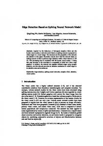
4.2 Edge Detection In this experience, we have chosen an image of a microscopic cell [31] defined on a pixel grid of 200 × 200 pixels (cf Fig. 14). To extract morphological features about nuclei from microscopy cellular image, it is usually required to find the edges of nuclei at first. In cellular imaging, it is important to analyze nucleus morphology by tracking its boundary, shape [32]. In this section, we focus on finding the boundary of nuclei by edge detection. Once the boundaries of nuclei are found, more features can be extracted about the nuclei, such as their form factor, convexity, compactness, and roundness. First image of a microscopic cell is segmented with spiking neural network, we have fixed the number of output neurons at 5, the step of training to 0.35, the choice of the base of training is random starting from the image source of 5% and numbers of receiving fields is 8 for each neuron in input, and the number of sub-synapses at 12. The image result obtained is shown in Fig. 15. Once the segmentation done, we will record the activity of each output neuron which gives for each input pixel an output binary 1 if the neuron is active or 0 if the neuron is inactive. The result of binary matrices activation of output neurons can be represented by binary images containing the edges detected by these neurons for each class (Fig. 16). Fusion is then made to have the final edge by superimposing the resulting images. The result of edge detection and a comparison with other methods of edge detection is obtained in Fig. 17.
123
B. Meftah et al.
Fig. 16 SNN edge network topology
Fig. 17 a Edge detection with Prewitt, b edge detection with morphology black top hat, c edge detection with Canny and d edge detection with SNN
5 Conclusion In this paper, we have applied a SNN model for image segmentation and edge detection. To use a SSN for both these problems, we have addressed the issue of parameter selection. We have focused our study on the key parameters: network architecture (number of subsynapses, receptive fields, output neurons) and learning parameters (training step, size of
123
Segmentation and Edge Detection Based on Spiking Neural Network Model
the training data base, peak of the learning function). These parameters are set up for each specific image problems. Results have shown that a careful setting of parameters is required to obtain efficient results. Future works will concern the application of this works to image sequences. References 1. Tavares JM (2010) A review of algorithms for medical image segmentation and their applications to the female pelvic cavity. Comput Methods Biomech Biomed Engin 13(2):235–246 2. Liew AW, Yan H, Law NF (2005) Image segmentation based on adaptive cluster prototype estimation. IEEE Trans Fuzzy Syst 13(4):444–453 3. Deng Y, Manjunath BS (2001) Unsupervised segmentation of color texture regions in images and video. IEEE Trans Pattern Anal Mach Intell 23(8):800–810 4. Senthilkumaran N, Rajesh R (2009) Edge detection techniques for image segmentation and a survey of soft computing approaches. Int J Recent Trends Eng 1(2):250–254 5. Freixenet J, Munoz X, Raba D, Marti D, Cufi X (2002) Yet another survey on image segmentation: region and boundary information integration. In: ECCV 2002. LNCS, vol 2352. Springer, Heidelberg, pp 408–422 6. Melkemi KE, Batouche M, Foufou S (2006) A multiagent system approach for image segmentation using genetic algorithms and extremal optimization heuristics. Pattern Recogn Lett 27(11):1230–1238 7. Xu C, Pham D, Prince J (2000) Image segmentation using deformable models. In: Fitzpatrick JM, Sonka M (eds) Handbook of medical imaging. Medical image processing and analysis, vol 2, SPIE Press, pp 129–174 8. Ghosh-Dastidar S, Adeli H (2009) Third generation neural networks: spiking neural networks. Adv Comput Intell AISC(61):167–178 9. Paugam-Moisy H, Bohte SM (2009) Computing with spiking neuron networks. In: Kok J, Heskes T (eds) Handbook of natural computing (40 pages—to appear). Springer Verlag, Heidelberg 10. Thorpe SJ, Delorme A, VanRullen R (2001) Spike-based strategies for rapid processing. Neural Netw 14(6–7):715–726 11. Wu QX, McGinnity M, Maguire LP, Belatreche A, Glackin B (2008) Processing visual stimuli using hierarchical spiking neural networks. Neurocomputing 71(10–12):2055–2068 12. Girau B, Torres-Huitzil C (2006) FPGA implementation of an integrate-and-fire LEGION model for image segmentation. In: European symposium on artificial neural networks ESANN’2006, Bruges, Belgium 26– 28 April 2006, pp 173–178 13. Buhmann J, Lange T, Ramacher U (2005) Image segmentation by networks of spiking neurons. Neural Comput 17(5):1010–1031 14. Rowcliffe P, Feng J, Buxton H (2002) Clustering within integrate-and-fire neurons for image segmentation. In: Artificial neural networks ICANN 2002, Madrid, Spain, 28–30 August 2002. LNCS, vol 2415. Springer, pp 69–74 15. Maass W (2001) On the relevance neural networks. MIT-Press, London 16. Gerstner W, Kistler WM (2002) Spiking neuron models, single neurons, populations, plasticity. Cambridge University Press, Cambridge 17. NatschlNager T, Ruf B (1998) Spatial and temporal pattern analysis via spiking neurons. Netw Comp Neural Syst 9(3):319–332 18. Averbeck B, Latham P, Pouget A (2006) Neural correlations, population coding and computation. Nat Rev Neurosci7:358–366 19. Stein R, Gossen E, Jones K (2005) Neuronal variability: noise or part of the signal?. Nat Rev Neurosci 6:389–397 20. Dayan P, Abbott LF (2001) Theoretical neuroscience: computational and mathematical modeling of neural systems. The MIT Press, Cambridge 21. Butts DA, Weng C, Jin J, Yeh C, Lesical NA, Alonso JM, Stanley GB (2007) Temporal precision in the neural code and the timescales of natural vision. Nature 449:92–95 22. Bohte SM (2004) The evidence for neural Information processing with precise spike-times: a survey. Nat Comput 3(2):195–206 23. Bohte SM, La Poutre H, Kok JN (2002) Unsupervised clustering with spiking neurons by sparse temporal coding and multi-layer RBF networks. IEEE Trans Neural Netw 13(2):426–435
123
B. Meftah et al. 24. Oster M, Liu SC (2004) A winner-take-all spiking network with spiking inputs. In: Proceedings of the 11th IEEE international conference on electronics, circuits and systems (ICECS 2004), Tel-Aviv, Israel, 13–15 December 2004, vol 11, pp 203–206 25. Gupta A, Long LN (2009) Hebbian learning with winner take all for spiking neural networks. In: IEEE international joint conference on neural networks (IJCNN), pp 1189–1195 26. Gerstner W, Kistler W (2002) Mathematical formulations of Hebbian learning. Biol Cybernet 87: 404–415 27. Leibold C, Hemmen JL (2001) Temporal receptive fields, spikes, and Hebbian delay selection. Neural Netw 14(6–7):805–813 28. Simoes AS, Reali Costa AH (2008) A learning function for parameter reduction in spiking neural networks with radial basis function. In: Proceedings of the 19th symposium of artificial intelligence (SBIA 2008), Savador, Brazil, 26–30 October 2008. Proceedings, vol 5249. Springer, pp 227–236 29. Martin D, Fowlkes C, Tal D, Malik J (2001) A database of human segmented natural images and its application to evaluating segmentation algorithms and measuring ecological statistics, In: Proceedings of the 8th international conference on computer vision, Vancouver, British Columbia, Canada, 7–14 July 2001, vol 2, pp 416–423 30. Meftah B, Benyettou A, Lezoray O, Wu QX (2008) Image clustering with spiking neuron network. In: IEEE world congress on computational intelligence, international joint conference on neural networks (IJCNN’08), Hong Kong, 1–6 June 2008, pp 682–686 31. Meurie C, Lezoray O, Charrier C, Elmoataz A (2005) Combination of multiple pixel classifiers for microscopic image segmentation. IASTED Int J Robot Auto 20(2):63–69 32. Chicurel M (2002) Cell migration research is on the move. Science 295:606–609
123