IEEE TRANSACTIONS ON MAGNETICS, VOL. 48, NO. 2, FEBRUARY 2012
223
Segmented-Locally-One-Dimensional-FDTD Method for EM Propagation Inside Large Complex Tunnel Environments Md. Masud Rana and Ananda Sanagavarapu Mohan School of Electrical, Mechanical and Mechatronic Systems, Faculty of Engineering and Information Technology, University of Technology Sydney (UTS), Sydney, Australia We propose a novel segmented locally one dimensional finite difference time domain (S-LOD-FDTD) method for modeling the electromagnetic wave propagation inside electrically large tunnels. The proposed S-LOD-FDTD method reduces the computational resources by dividing the problem space into segments. To validate this method, we simulate the propagation in real tunnels and compare the results with the published measured data. The comparisons reveal that the proposed method can predict the fields accurately in real, large tunnels at longer ranges with significant savings in execution time and memory. Index Terms—EM propagation, LOD-FDTD, path loss, segmented LOD-FDTD, tunnels.
I. INTRODUCTION
R
ADIO wave propagation inside tunnels, traditionally has been modelled using such techniques as modal analysis, geometrical optics and the parabolic equation (PE) approximation [1]–[3]. The FDTD method has also been used extensively for modeling radio wave propagation inside tunnel environments. But for modeling electrically large tunnels, FDTD requires excessive memory and CPU resources. To ease the computational burden of FDTD, many techniques have been proposed. Chevalier and Inan [4] proposed the segmented long path propagation (SLP) technique to reduce the computational load for long ionospheric propagation using FDTD and FDFD. Most recently, Segmented Finite Difference Time Domain (S-FDTD) method was introduced for reducing the computational requirements for solving propagation in electrically large tunnels [5]. However, the S-FDTD method, inherits the limitations of the conventional FDTD method, due to the Courant-Friedrichs-Lewy (CFL) stability constraint, which would still require large number of segments leading to increased computational load when solving for electrically large tunnels. To overcome these limitations, the alternating direction implicit FDTD (ADI-FDTD) method was proposed [6]–[8]. Recently, segmentation approach was also extended for ADI-FDTD for modeling propagation inside tunnels [9]. However, the S-ADI-FDTD method still suffers from limitations due to higher Courant-Friedrichs-Lewy numbers (CFLN) for solving electrically large problems. CFLN is defined by where is determined from CFL condition. To overcome these problems, Locally-One-Dimensional FDTD (LOD-FDTD) was proposed [10], [11]. But the direct application of LOD-FDTD method for solving electrically large tunnels would still require huge computational resources as it has to solve sets of the simultaneous equations. Therefore, methods to overcome the limitations of LOD-FDTD method to solve for electromagnetic propagation in large sized tunnels are desirable.
Manuscript received July 07, 2011; revised October 06, 2011; accepted November 04, 2011. Date of current version January 25, 2012. Corresponding author: M. M. Rana (e-mail:
[email protected]). Color versions of one or more of the figures in this paper are available online at http://ieeexplore.ieee.org. Digital Object Identifier 10.1109/TMAG.2011.2177075
In this paper, we propose the Segmented-LOD-FDTD method for solving the electromagnetic wave propagation inside electrically large tunnels. In the proposed S-LOD-FDTD method, larger time step size can be used for overcoming the CFL stability constraint. Thus, the proposed method can ease the demands on computational resources and improves the feasibility of running large scale numerical electromagnetic simulations on a standard PC. II. FORMULATION OF S-LOD-FDTD METHOD A. Segmented-LOD-FDTD Method To apply the proposed S-LOD-FDTD method, we break up the computational space into segments and use LOD-FDTD and Convolutional Perfectly Matched Layer (CPML) absorbing boundary conditions for each segment and solve them sequentially. Fig. 1 schematically represents the 2-D computational space for a general rectangular tunnel with a branch where rectangular segments represent sequential 2-D LOD-FDTD spaces in which electromagnetic fields from a transmitter to the receiver are calculated. In general, the computational domain is divided into a number of individual segments each with equal or variable segment lengths depending on the shape of the tunnel so that different types of tunnels such as branched or curved tunnels can be modelled. Whenever there are abrupt changes in tunnel geometries (see Fig. 1), the boundaries must be carefully treated so as to compute the fields accurately. The proposed S-LOD-FDTD algorithm is summarized as follows: 1) Start the conventional LOD-FDTD iteration with CPML absorbing boundary condition in first segment when the signal source S0 is provided. 2) When the fields of the segment 1 reaches its steady state at each unit cell on the interface 1, save the electric and magnetic fields from each unit cell recorded at the interface 1 for use in the next segment. ’ on the left side 3) Referring to Fig. 1, the fields from ‘ of interface 1 are saved from Segment 1 and used as input ’ that is lying on the right side of the interface fields in ‘ which then feeds Segment 2 and so on. 4) Whenever an abrupt change or branching junction falls within a segment, its effect on the fields needs to be considered before propagating the signal into next segment. 5) Sequentially propagate the extracted fields at the interface into next segment.
0018-9464/$31.00 © 2012 IEEE
224
IEEE TRANSACTIONS ON MAGNETICS, VOL. 48, NO. 2, FEBRUARY 2012
Fig. 1. 2-D segmented problem space in S-LOD-FDTD method for branched tunnel.
Follow the above steps to complete the simulations in seg. In the following section, LOD-FDTD ments method and CPML for each segment are described. B. LOD-FDTD Method in Each Segment To apply the locally one dimensional finite-difference timedomain (LOD-FDTD) algorithm [11] for each discrete time step waves is requires two procedures. The first procedure for shown below. Sub-step 1:
C. CPML Absorbing Boundary Condition in Each Segment In LOD-FDTD method, similar to ADI-FDTD [1], [6]–[8]. the boundary condition for the intermediate plane is considered same as those for physical planes so that a first order overall accuracy can be obtained. For the sake of brevity, here we provide limited details for deriving CPML where the electric and magnetic fields are obtained as: Sub-step 1:
(1a)
(3a)
(1b) where and spatial step of
are the fields in a discrete grid sampled with a . Placing (1a) in (1b) yields
(2)
(3b) and are discrete variables which may have where non-zero values only in some CPML regions but are necessary to implement the absorbing boundary [11]. In order to avoid reflections between the computational domain and the CPML boundary due to the discontinuities, the losses due to the CPML must be made zero at the interfaces of the computational domain. III. RESULTS USING S-LOD-FDTD METHOD
where A. Straight Tunnel
The simultaneous linear equations in (2) can be rewritten in the tri-diagonal matrix form. Similarly, for the second step, the equations can also be developed.
In this paper, at first, we consider the Roux tunnel [2] which is perfectly straight and has a length of 3.336 km as shown in Fig. 2(a). The origin of the tunnel-coordinate system is arranged to be at the centre of the tunnel cross section. The transverse section is semicircular as shown in Fig. 2(b) and has a diameter of 8.3 m, the maximum height is 5.8 m at the centre of the tunnel with material properties and . The predicted path loss in this tunnel (for a length of 500 m) at 2.4 GHz computed using proposed S-LOD-FDTD is shown in Fig. 2(c)
RANA AND MOHAN: SEGMENTED-LOCALLY-ONE-DIMENSIONAL-FDTD METHOD FOR EM PROPAGATION
Fig. 2. (a) Roux tunnel, (b) Profile of the Roux tunnel, (c) Comparison with measured data of E. Masson et al.
225
Fig. 5. (a) Geometry of the branched tunnel, (b) Comparison with the measured data of Zhang et al.
Fig. 6. (a) Geometry of curved tunnel (b) Segmented problem space of the curved tunnel.
B. Branched Tunnel Fig. 3. Comparison of averaged (over 50 m) path loss for Roux Tunnel.
Fig. 4. (a) Cross section of the Massif Central tunnel, (b) Simulated and measured electric field intensity.
along with the measured data extracted from publication by E. Masson et al. [2] to make a comparison. Fig. 3 shows a comparison of the averaged path loss obtained for Roux tunnel in which the measured results extracted from the published graphs in [2] were averaged over 50 m length and compared with the averaged simulated data. Next, we consider the Massif Central tunnel which is also a straight tunnel that is 3.5 km long and compare the results obtained from proposed S-LOD-FDTD with measurements provided by Dudley et al. [3]. The measurement cross section of Massif tunnel is shown in Fig. 4(a) and the electrical characteristics of the tunnel wall are and . The predicted field intensity (for a length of 2500 m) at 450 MHz as a function of axial distance is compared with the measured data that was extracted from [3] and shown in Fig. 4(b). The cell size chosen for both the and a CFLN of 2 chosen for the Roux tunnel problems is whereas CFLN of 4 for the Massif tunnel. For the Roux tunnel, the execution time required by the S-ADI-FDTD method was 5.3 hrs. with a memory over 5 MB whereas the S-LOD-FDTD took 2.86 hrs with a memory of 950 KB. Comparison in terms of execution time and memory shows that S-LOD-FDTD is more effective as it requires less time and memory.
Here, we consider a branched tunnel that is similar to the geometry published in Zhang et al. [12] and compare our S-LODFDTD simulations with their measurement data. The two dimensional geometry of the tunnel shown in Fig. 5(a) was approximated from the 3-D tunnel geometry published in Zhang et al. [12] and the electrical parameters of the tunnel are chosen to be same as those given in [12] for comparing the results. The transmitter is positioned in the main section at a distance of 10 m away from the junction formed by the branch and main sections of the tunnel at an angle of 15 . The receiver is assumed to move away from the transmitter into the branch section assuming TM incidence. The segment length of 20 m is considered for both the branch and main sections. The electrical characteristics of the tunnel wall are and . Fig. 5(b) shows that the path loss obtained in the branch tunnel by the proposed method as compared with the published measured data given in [12]. The execution time and memory required for S-LOD-FDTD are 40 min and 3.9 KB for a . C. Curved Tunnel Finally, we present results for a curved tunnel with a straight entrance using the proposed method and compare them with published measured data given in [13]. For the simulation of the curved tunnel geometry as shown in Fig. 6, same parameters as given in [13] were chosen. The width and heights of the tunnel cross section are 8 and 6 m respectively and the transmitter and receiver are centered in the tunnels with their heights above the ground being 3 and 1.5 m, respectively. The electrical characteristics of the tunnel wall are and . Uniform segmentation was considered for the straight segment of the curved tunnel. But for the curved segment, the slope at each segment interface must be determined which needs to be multiplied with the fields calculated for the previous segment before propagating them into the next segment. The axial length of the curved tunnel is 400 m and the length of the curved section is 200 m. and a segment length of 25 m was considered. Fig. 7 shows the predicted path loss at
226
IEEE TRANSACTIONS ON MAGNETICS, VOL. 48, NO. 2, FEBRUARY 2012
Fig. 7. Comparison with measured received power along the propagation axis of curved tunnel. TABLE I REQUIRED COMPUTATIONAL TIME AND MEMORY USING S-LOD-FDTD METHOD FOR ROUX TUNNEL (CFLN = 2)
1 GHz that is compared with the measured data extracted from [13]. Table I summarizes the computational performance in terms of execution time and memory of the proposed S-LOD-FDTD method for Roux tunnel for different segment sizes. The tabulated results indicate that by dividing the domain into more segments, both execution time and memory usage can be reduced. However, the segment size cannot be reduced to be arbitrarily small in order to obtain further improvements. It was observed for the case of Roux tunnel, that when the size of the segment falls below 10 m, the results became unstable. This was because the total number of time steps iterated in each segment was not sufficient for the solution to reach its steady state for that segment length. So for electrically large Roux tunnel, considering the stability of the solution, the S-LOD-FDTD obtained maximum time and memory savings for 50 equal sized segments with each segment having a length of 10 meters. The relationship between the total CPU execution time and segment size is given in [5]. The dispersion error for different CFLN is shown in Fig. 8(a). In this paper a maximum is used for calculations. Fig. 8(b) shows the relative errors of the S-LOD-FDTD method with respect to CFLN. The relative error is calculated using the following formula:
Where
is the reference value (standard FDTD) and is the calculated value using S-LOD-FDTD. From Figs. 8(a) and (b), it can be observed that the dispersion and relative errors increase with the increasing CFLN, however, the maximum error is only around 4%. The results confirm that the proposed S-LOD-FDTD method is computationally more efficient and provides accurate results for two dimensional propagation predictions inside large tunnels.
Fig. 8. (a) Normalized phase velocity vs. wave angle for different CFLN (b) Relative error with respect to CFLN.
IV. CONCLUSION In this paper, we propose a new two dimensional Segmented-LOD-FDTD method for propagation prediction inside large straight, branched and curved tunnels. The results indicate higher signal attenuation for the junction/transition regions as compared to regions away from such abrupt transitions. The predictions on path loss agree reasonably well with published measured data. The results reveal that the proposed segmentation approach can help to reduce the computational resources and hence can be extended for electromagnetic modeling of any long path propagation problems. REFERENCES [1] R. Martelly and R. Janaswamy, “An ADI-PE approach for modeling radio transmission loss in tunnels,” IEEE Trans. Antennas Propag., vol. 57, no. 6, pp. 1759–1770, 2009. [2] E. Masson, P. Combeau, M. Berbineau, R. Vauzelle, and Y. Pousset, “Radio wave propagation in Arched cross section tunnels-simulations and measurements,” J. Commun., vol. 4, no. 4, pp. 276–283, 2009. [3] D. G. Dudley, M. Lienard, S. F. Mahmoud, and P. Degau-que, “Wireless propagation in Tunnels,” IEEE Antennas Propag. Mag., vol. 49, no. 2, pp. 11–26, 2007. [4] M. W. Chevalier and U. S. Inan, “A technique for efficiently modeling long path propagation for use in both FDTD and FDFD,” IEEE Antennas Wireless Propag. Lett., vol. 5, no. 1, pp. 525–528, 2006. [5] Y. Wu and I. Wassell, “Introduction to the segmented finite-difference time domain method,” IEEE Trans. Magn., vol. 45, no. 3, pp. 1364–1367, 2009. [6] O. Ramadan, “Complex envelope four-stage ADI-FDTD algorithm for narrowband electromagnetic applications,” IEEE Antennas, Wireless Propag. Lett., vol. 8, pp. 1084–1086, 2009. [7] D. L. Sounas, N. V. Kantartzis, and T. D. Tsiboukis, “Optimized ADIFDTD analysis of circularly polarized microstrip and dielectric resonator antennas,” IEEE Microw. Wireless Compon. Lett., vol. 16, no. 2, pp. 63–6, Feb. 2006. [8] T. Stefanacuteski and T. D. Drysdale, “Parallel implementation of the ADI-FDTD method,” Microw. Optical Technol. Lett., vol. 51, no. 5, pp. 1298–1304, May 2009. [9] M. Rana and A. S. Mohan, “EM Propagation modeling in complex tunnel environments,” in Proc Asia Pacific Symp. Applied Electromagnetics and Mechanics (APSAEM), Kuala Lumpur, Malaysia, Jul. 28–30th, 2010, pp. 396–401. [10] V. Nascimento, B. Borges, and F. L. Teixeira, “Split-field PML implementations for the unconditionally stable LOD-FDTD method,” IEEE Microw. Wireless Compon. Lett., vol. 16, no. 7, pp. 398–400, Jul. 2006. [11] I. Ahmed, E. P. Li, and K. Krohne, “Convolutional perfectly matched layer for an unconditionally stable LOD-FDTD method,” IEEE Microw. Wireless Compon. Lett., vol. 17, no. 2, pp. 816–818, 2007. [12] Y. P. Zhang, Y. Hwang, and R. G. Kouyoumjian, “Ray-optical prediction of radio-wave propagation characteristics in tunnel environmentspart 2: Analysis and measurements,” IEEE Trans. Antennas Propag., vol. 46, no. 9, pp. 1337–1345, Sep. 1998. [13] T. Wang and C. Yang, “Simulations and measurements of wave propagations in curved road tunnels for signals from GSM base stations,” IEEE Trans Antennas Propag., vol. 54, no. 9, pp. 2577–2584, 2006.