Selecting Key Features for Remote Sensing Classification by Using ...

Selecting Key Features for Remote Sensing Classification by Using Decision-Theoretic Rough Set Model Feng Xie, Dongmei Chen, John Meligrana, Yi Lin, and Wenwei Ren

Abstract There are many spectral bands or band functions developed for land-cover feature measurements. When the ratio of the number of training samples to the number of feature measurements is small, the traditional land-cover classification is not accurate. To solve this problem, a decision-theoretic rough set model (DTRSM) is first introduced. This model is linked with distinguishing different types of samples in the image. The samples in the minority classes will be misclassified based on the model. To minimize the misclassification, we propose an improved feature selection algorithm with comprehensive criteria. This algorithm is implemented on the Landsat TM data covering two disparate regions which are Lake Baiyangdian and Lake Qingpu located in the north and south of China, respectively. We compare the algorithm with other feature selection algorithms. Results show that the proposed method can effectively select key features for different data sets and the accuracy of classifiers can be ensured.

Introduction With the availability of remotely sensed data with increasing spectral bands collected by different sensors, the classification of these data by conventional classifiers may suffer from Hughes phenomenon: As the number of spectral bands or band functions increase, the classification accuracy can decrease with a fixed number of training samples (Shashahani and Landgrebe, 1994). In classification, class conditional probability density functions (PDFs) need to be estimated from a set of training samples. When these estimates are substitute for the true values of the PDFs, the resulting classification is suboptimal and hence has a higher probability of error. When

Feng Xie is with the School of Urban Rail Transportation, Soochow University, Suzhou 215131, China. Dongmei Chen is with the Department of Geography, Queen’s University, Kingston, ON K7L3N6, Canada. John Meligrana is with the School of Urban and Regional Planning, Queen’s University, Kingston, ON K7L4R2. Yi Lin is with the Research Center of Remote Sensing and Spatial Information Technology, Tongji University, Shanghai 200092, China. Wenwei Ren is with the Key Laboratory of Yangtze River Water Environment, Ministry of Education, College of Environmental Science and Engineering, Tongji University, Shanghai 200092, China, and also with the Ministry of Education Key Laboratory for Biodiversity Science and Ecological Engineering, School of Life Sciences, Fudan University, Shanghai 200433, China ([email protected]). PHOTOGRAMMETRIC ENGINEERING & REMOTE SENSING

a new additional feature is added to the data, the bias of the classification error increases because more parameters of PDFs need to be estimated from the same number of samples. This is so called the Hughes phenomenon. Training samples are needed for all ground cover classes of interest. A good training sample can represent a kind of land-cover type, which shed light on environmental and ecological issues (Binford et al., 2004; Li, 2006; Pielke, 2005). The number of training samples is closely related to the classification complexity (Hu et al., 2007; Pan and Billings, 2008; Yu and Liu, 2004). In practice, we often cannot find enough number of training samples of minority land-cover classes in a scene. In any case, the process of acquiring training samples is usually expensive or time consuming, and only a limited number of training samples can be obtained (Shashahani and Landgrebe, 1994). When the number of training samples is small compared to the dimensionality (feature measurements) of the data, the Hughes phenomenon is emerging. This is also called the “curse of dimensionality” in the field of pattern recognition (Duda et al., 2001; Friedman, 1997; Jain and Zongker, 1997; Yang and Honavar, 1998). To solve this problem, we expect to select key features from a large number of bands or band functions that can effectively reduce the dimensionality of the data for the following classification. Feature selection can rely on the electromagnetic characteristics of ground objects. Lee (2009) selected a narrowband model to wideband data and found that the mismatch could result in a >20 percent underestimation in calculating reflectance. Some mathematical transformation methods were used to find the main features of objects. Kalelioglu et al. (2009) used principal components analysis (PCA) and Crosta techniques to analyze the Landsat-5 Thematic Mapper (TM) images and selected PCA123 image, RGB731, and TM band ratio (band5/ band7, band5/band1) to discriminate the dyke boundaries. PCA is a linear transformation as preliminary step for decorrelation or denoise and cannot handle a nonlinear system correctly. Furthermore, classification is not considered in PCA where the most divergence is not the most advantage for discrimination. These methods are often used as the preliminary steps for reducing correlation among features and can be easily disturbed by outliers (Jolliffe, 2002; Shlens, 2005). Feature selection can also be conducted through searching algorithms. Metaheuristic algorithms including trajectory and population-based algorithms have been proposed to Photogrammetric Engineering & Remote Sensing Vol. 79, No. 9, September 2013, pp. 000–000. 0099-1112/13/7909–0000/$3.00/0 © 2013 American Society for Photogrammetry and Remote Sensing September 2013

1

find optimal subsets of features. Simulated annealing and Tabu search methods are examples of traditional trajectory methods (Glover and McMillan, 1986; Granville et al., 1994; Kirkpatrick et al., 1983), and genetic algorithms are examples of the most known population-based methods (Muni et al., 2006; Oh et al., 2004; Yang and Vasant, 1998). Although there are a lot of these searching algorithms, greedy searching strategies which make a “greedy” choice (locally optimal choice) in the hope that this choice will lead to a globally optimal solution (Cormen et al., 2009) seem to have the advantages of computation and robustness against overfitting-based as seen in many previous studies (Chow et al., 2008; Hu et al., 2010; Hu and Cercone, 1995; Mitra et al., 2002; Torkkola, 2003; Xie et al., 2011). Xie et al. (2011) implemented a forward greedy searching algorithm (FGSA) by applying a variable precision rough set (VPRS) model in selecting important features to distinguish different reed communities and water bodies from Landsat imagery. Due to the partial (probabilistic) “inclusion” or “belonging to” concept, VPRS is preferred in dealing with the confusing “different objects/same images” phenomenon of remote sensing. The major advantages of VPRS include allowing the classification with a controlled degree of uncertainty, or a misclassification error, and introducing a parameter to control the noise effect as illustrated by previous studies (Beynon, 2001; Dimitras et al., 1999; Xie et al., 2011). VPRS can be derived from the Decision-Theoretic Rough Set Model (DTRSM) based on a theoretic framework (Yao and Zhao, 2008). Few studies have applied DTRSM in the remote sensing field. Feature evaluation is a crucial step in feature selection (Jain and Zongker, 1997; Quafafou and Boussouf, 1997; Zhao et al., 2006). Evaluation criteria play a pivotal role in applying DTRSM. Although some researchers have evaluated features based on the rate of class-undetermined samples over the entire sample set (Hu et al., 2008; Hu and Cercone, 1995; Jensen and Shen, 2004), this rate is too simple to identify the real source of error resulting in misclassification. Yao and Zhao (2008) suggested that feature selection should consider one or more criteria in theory, but did not show how to undertake this in practice. In this article, we implement a comprehensive set of criteria involving confidence, cost or lost, and generality in the procedure of feature selection. This paper mainly focuses on how to set comprehensive evaluation criteria in a FGSA for feature selection based on DTRSM to minimize misclassification errors that will be evoked by classifiers. The paper is organized as follows. In the next Section, the theory of DTRSM used is introduced and discussed. Based on the analysis of real source of discrimination error, three criteria are proposed in relation to the Bayes error rate of classification. Then, the method implemented in remote-sensing practice and applied in the case of two disparate ground objects d in the north and south of China, respectively, is presented. When the confidence level is determined, only one parameter needs to be set in our method. Next, we emphasize on how to set this parameter and compare the accuracy through applying different classification algorithms on different data sets, including derived from other feature selection algorithms. After analysis, our summary concludes that the proposed method can effectively reduce the complexity of data sets and guarantee the accuracy of any classifiers.

Theories and Preliminary Work Decision-Theoretic Rough Set Model The DTRSM was proposed in the early 1990s based on the well-established Bayesian decision procedure, which deals with making decisions with minimum risk based on observed evidence (Yao, 2008; Yao and Zhao, 2008). DTRSM can derive 2

September 2013

probabilistic and classic rough set models, including VPRS and Pawlak rough set. We will link this model with remote sensing classification in this section. There are three regions (the positive region, the boundary region, and the negative region) that can be used to for assigning pixels or objects of the remotely sensed image (I) into a land cover class (Set X) based on an equivalent relation set (A) formed by all the features of objects (pixels also can be seen as objects) in the image. We can randomly select some features from set A to build subset B which obeys the indiscernibility relation IND(B), that is: IND N ( B ) = { x , y > ∈I × I ∀a

B,a , a( x ) a( y )}, ∀ B ⊆ A

(1)

where, x and y are objects in the image (I ), < x, y > ∈ IND(B) means x and y are indiscernible with respect to subset B (a feature set). Two objects in the image satisfy indiscernibility relation if and only if they have the same values on all features in B. The indiscernibility relation is an equivalent relation because it satisfies the properties of reflexivity, symmetry and transitivity. Then, the equivalent class induced by IND(B) (hereafter B for short) is: [

]

i B

{

i,j

, < xi ,

j

( B )}

(2)

where, xi and xj are objects in the image (I). If [xi]B is definitely a part of Set X (projected to a landcover class), that is, the lower approximation BX : BX = {[ x i ]B [ x i ]B ⊆ X , x i ∈ I }.

(3)

If the intersection of [xi]B and X is non-empty, that is, the upper approximation BX : BX = {[ x i ]B [ x i ]B I X ≠ ∅, x i ∈ I }

(4)

From Equations 3 and 4, it is seen that BX X BX . If and only if BX = BX , the remotely sensed data, can be definitely classified by B features without error. In practice, BX is not equal with BX that means there are misclassification by using B features. The elements of remotely sensed data in BX which definitely belong to a ground cover class form the positive region BX which definitely do of X. The elements in the set of I B not belong to the class form the negative region of X. Then, N ( X ) = BX − BX ; it contains the the boundary region is BND elements whose belongings are undetermined. The defect of the Pawlak classic rough set model is that it does not consider the degree of overlapping feature measurements (e.g., band values), whereas, the probabilistic approaches established on probabilistic positive, boundary, and negative regions have considered the overlapping features by using threshold parameters. If the degree of overlapping feature measurements is larger than a threshold, the objects with these features are in the probabilistic positive region of a land-cover class. If the degree of overlapping is lower than another threshold, the objects are in the probabilistic negative region of the class, and if the degree is between these two parameters, the objects are in the boundary region of the class. How to determine this pair of parameters is a critical question and when they are computed from risk or loss function based on the Bayesian decision procedure, then this model is DTRSM. Minimizing the Probability of Classification Error According to three regions for approximating land-cover classes, objects which have the same feature measurements but belong to different classes (class X and not X) cause confusion in classification and will be assigned to the boundary region of X. Not all elements (representing objects) in the PHOTOGRAMMETRIC ENGINEERING & REMOTE SENSING

boundary region of X will be misclassified (Hu et al., 2007). Only the elements that do not belong to the majority class in the boundary region will be misclassified based on the Bayes rule. Minimizing misclassification is naturally related to the Bayes error rate (Peng et al., 2005). In the multiclass case, there are more ways to be wrong than to be right, therefore, it is simpler to compute the probability of being correct (P(correct)), which is presented by Equation 5: C

P (correct r )=

∑ P( i =1

C

Ri ,

i

)

∑ ∫ p(

)P (␻i )dx

(5)

i =1 Ri

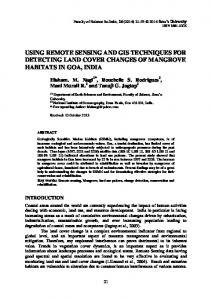
where ωi is a land-cover class i, x is an object in the image, p( i ) is the conditional probability density function, c is the number of all land-cover classes, and Ri is the region caused by the decision point (Duda et al., 2001). P(ωi) and p( i ) are unknown in the real world, and it is not feasible to estimate them in the high-dimensional feature space when there are few training samples. To make this easier to understand, we describe it as follows. The remotely sensed image can be seen as a discrete space where samples in the image are divided into a feature set {E1, E2,…, EK} based on the responses of different ground objects. The samples with the same measured values are grouped into the same feature. As shown in Figure 1, the height of the rectangle denotes the probability p (Ei) of feature Ei. The pure

feature refers to the samples with this feature belong to unique land-cover, such as E1, E2, E5, or E6 in Figure 1. Impure feature refers to the samples with this feature actually belong to two (or more) ground covers, such as E3 or E4. Estimating the percentages of impure features is important for control classification error. Many measures have been developed, such as distance (Ho and Basu, 2002; Robnik-Sikonja and Kononenko, 2003), mutual information (Battiti, 1994), correlation (Guyon and Elisseeff, 2003), dependency (Jensen and Shen, 2004), consistency (Dash and Liu, 2003), and neighborhood decision error rate (NDER) (Hu et al., 2010). Because distance, mutual information, and correlation measures have little relationship with the boundary region, they are not suitable for estimating. The measure of dependency is commonly used. An equation for dependency is:

␥C =

POSC ( D )

(6)

I

where |·| denotes the cardinality of the set; POSC(D) is a positive region; A = C U D, C and D are named as the condition set C and decision set D , respectively (Pawlak and Skowron, 2007), and I means the image. Equation 6 reflects a ratio of objects with pure features over all objects in the image. It does not take the objects with impure features that exist in the boundary regions of classes into account. Thus, the dependency measure is also not a good measure. Some other measures were developed after dependency. For instance, consistency as a coverage measure was introduced and employed to evaluate the importance of features in a discrete case (Dash and Liu, 2003; Kohavi and John, 1997). NDER was defined as an estimate of the classification complexity in Hu et al. (2010). These studies suggest that a good measure should consider the objects with impure features in the boundary regions of classes. A Comprehensive Set of Criteria To minimize the probability of classification error, we need measure the objects with impure features (e.g., E3 and E4 in Figure 1) in the boundary regions of classes. According to the Bayes’ rule, the objects in a boundary region of a landcover class X are in either of two complement states: grouped to a decision class (X) or not to (¬X). The probabilities for these two complement states are denoted in the following equations: P ( X [ x ]R ) =

X I [ x ]R [ x ]R

,

P ( X [ x ]R ) = 1 −

X I [ x ]R [ x ]R

(7)

where, R is ∪Ri, an equivalent relation set formed by the features of objects. With respect to the three regions (the positive region, the boundary region, and the negative region), there are three actions to classify the objects into any of them, i.e., aP, aB, aN. When an object belongs to the land-cover class X, let λPP, λBP, and λNP denote the costs of taking the action aP, aB, and aN, respectively; when it does not belong to X, let λPN, λBN and λNN denote the costs of taking the same three actions. Then the cost function (fcost) of taking action {aP, aN, aB} with respect to the three regions can be expressed as: Figure 1. Discrete decision system of remote sensing. By comparing (a) and (b), although the probabilities of impure features are identical, the probabilities of misclassification are different (adapted from Hu et al. (2010)).

fcos t aP [ x ]R ) ␭PP P(X P (X P( ( X [ x ]R ) + ␭PPN P ( X [ x ]R ) fcos t aB [ x ]R )

BP B

P P((X P(X ( X [ x ]R ) + ␭BBN P ( X [ x ]R ).

(8)

fcos t aN [ x ]R ) ␭NP P P((X P(X ( X [ x ]R ) + ␭NNN P ( X [ x ]R ) PHOTOGRAMMETRIC ENGINEERING & REMOTE SENSING

September 2013

3

The Bayesian decision procedure leads to the minimumrisk decision rule of the boundary region, that is: If fcos t aB [ x

R

fcos t (aP [ x ]R ) and fcos t aB [ x ]R )

fcos t aN [ x ]R ),

decide [ x ]R ⊆ BND( X )

(9)

where BND(X) denotes the boundary region of X. Because only the objects which belong to the minority classes in the boundary region cause error, the cost λBP is less than λBN. Given ␭BP = 0 and ␭BN = 1, then the cost function of taking action aB pertaining to the boundary region is:

fcos t aB [ x ]R ) P ( X [ x ]R ) = 1 − P ( X [ x ]R )

(10)

where P(X|[x]R) is the probability of x with the description [x]R belonging to the decision class X, that is: P ( X [ x ]R ) =

[ x ]R I X [ x ]R

= confid f ence ([ x ]R

X).

(11)

When confid f ence ([ x ]R X ) ≥ ␣, the quantity 1 − α becomes the error rate of classifying the objects to class X based on R feature set. The larger P(X|[x]R) has the higher probability of being majority class in the boundary region of land-cover class X, or vice versa. The smaller P(X|[x]R) has the higher probability of being minority class in the boundary region that always causes the error. Then, the following criterion needs to be satisfied: P ( X [ x ]R ) max P P(( x

R,

i

)

Method and Implementation DTRSM Applying in Remote Sensing The main aim of this session is to implement the DTRSM in remote sensing practice. Key features are selected for classification or ground object extraction from a number of features, including spectral bands, Ratio Vegetation Index, band math, etc., to avoid the effect of Hughes phenomenon. The flow diagram is shown in Figure 2. There are several main processes in this flowchart. First, we collect available data (e.g., spectral bands and maps) and register them into the same coordinate system. Second, we select plots that have typical land-covers of the region and can be easily accessed for in situ investigation and afterwards for validation. Next, we construct the condition set by various features (e.g., spectral bands, band math) and the decision set based on the reference data, that is, we identify the class labels of samples by manual work. Then, we link the condition set with decision set one-on-one based on the sequence of pixels in the image to form a table of training data classes and predictive data. A forward greedy searching algorithm (FGSA) improved by comprehensive criteria is created to handle this table based on the theories of DTRSM. This improved FGSA is

(12)

where ωi is the i(I = 1, 2, …, c) class; X is the decision class; the maximum P correspond to the largest probability of being majority class. Equation 12 means that the majority class in the boundary region is projected to the decision class. At the same time, if P ( X [ x ]R ) ≠ ax x P ( x ∈ R, i ), it suggests that the decision class corresponds to the minority class in the boundary region, which causes error. Thus, the loss function (floss) is as follows: ⎧0, P ( X [ x ]R ) ma P ( x R, ␻i ) ⎪ . (13) floss = ⎨ ⎪⎩1, P ( X [ x ]R ) ≠ max P ( x R, ␻i ) For all objects in the remotely sensed image, the total loss is: n

Tloss = ∑ floss. i=1

Finally, the improved γ measure proposed is: T ␥ = 1 − loss I

(14)

(15)

where |I| is the number of objects in the image. Equation 15 is a kind of generality measure based on Yao and Zhao’s theory (2008). More than just derived from the Bayes’ decision rule, the γ is improved by considering confidence, costs and risks, loss function, and generality comprehensively. Its advantages are as follows: 1. convenient for dealing with discrete and numerical data; 2. confidence guarantees it is tolerant to data with error in practice; and 3. costs and loss function measure the real source of classification error.

From the above deduction, a comprehensive set of criteria is proposed to minimize the error. From Equation 11, the confidence level (α) should be first guaranteed (Criterion I), then the loss (from Equation 13) is the lowest, that is to say, the highest generality (from Equation 15) correspond to the largest γ value (Criterion II). Besides, a feature is unnecessary if we add it into the feature set (R) with no change in γ (Criterion III). In the next section, we will show how to implement these criteria in the process. 4

September 2013

Figure 2. The flowchart of DTRSM for remote sensing classification. FGSA means forward greedy searching algorithm. The FGSA improved by comprehensive criteria is detailed in the following pseudo-code.

PHOTOGRAMMETRIC ENGINEERING & REMOTE SENSING

detailed following the flowchart. The output of FGSA is the set of key features. Algorithm: FGSA improved by comprehensive criteria Input: A table of linking the condition set with decision set by the sequence of image units Output: Set R containing key features Step1: ← ∅; Step2: for each ak ∈ C − R compute P ( X [ x ]{ a }UR ) ≥ ␣ ; k // Criterion I

/ / where, k

, ,..., , , C = U {ak }

Step 3: compute loss based on Eq. (13) and (14); Step 4: compute improved γk(k = 1, 2…) based on Eq. (15); Step 5: select am corresponds to the largest γm among γk; // Criterion II Step 6: if |γm − γ0| > Δ //// Criterion III

/ / the initial value of ␥ 0 is 0 / / ⌬ is a tthreshold of significance which is deterrmined by confidence level i ← i + 1; R ← R U {am };

␥0 ← ␥ m ; go to step 2; else return R; Step 7: end The functions of improved γ and Criterion I, II, and III are enforced in the process of the above algorithm. First, there is no feature in the set (R), i.e., R ← Ø. Second, the P ( X [ x ]{ a }UR ) k of every ak ∈ C − R(k = 1, 2…) is computed by Equation 11 with the confidence level α = 99% (Criterion I). Third, the total loss (Equation13 and 14) is calculated and the improved γk (k = 1, 2…) is obtained by Equation15 corresponding to each ak ∈

C − R (k = 1, 2…). The am corresponding to the largest γm among all γk values is selected to meet the Criterion II. If adding am to R leads to the change of γ over the threshold of significance Δ (|γm − γ0| > Δ, where the initial value of γ0 is 0 and Δ is determined by confidence level), am is an important feature which contains significant information not included in R. Then am is added into the R (R ← R ∪ {am}), and the γ0 is replaced by γm and the new loop begins. This program will not end until there is no or little change in γ when the Criterion I is reached. The highlight of the algorithm is the introduction of multiple criteria (Criterion I, II, and III) for minimizing the probability of error in decision. If key features are found in this process, they will be used in the following supervised classification. Case Studies Using remotely sensed imagery to gain insights into the terrestrial environment is necessary because many parts of nature are inaccessible or sensitive to human disturbance. Furthermore, in situ investigation or field survey of land-cover classes in the whole region are usually expensive and time consuming. Thus, remote sensing interpretation is desirable, and the above procedure is implemented in the following two cases. One case is Lake Baiyangdian (hereafter referred to as BYD) located near Beijing City in the north of China. Lake BYD is an excellent case to test our model because its fuzzy boundaries among different land-covers and water bodies are hard to distinguish in the remotely sensed image. Lake BYD is the largest freshwater lake of the North China Plain which is important for the regional wetland and water supply for Beijing metropolitan area. Another case is Lake Qingpu located near Shanghai Proper in the south of China. Lake Qingpu (QP) is selected as the case study as it has more balance of land-cover types and is also important for regional wetland protection and water supply for Shanghai metropolitan area. These two study areas both lie at water source areas for two mega-cities, Beijing and Shanghai, which enable comparisons between different land-cover types in north and south China (Plate 1).

Plate 1. The locations of two study areas: (a) True color image of Lake BYD near Lianggou village, (b) The reference image of Lake BYD near Lianggou village, (c)True color image of Qingpu (around Siqian village), and (d) The reference image of Qingpu (around Siqian village).

PHOTOGRAMMETRIC ENGINEERING & REMOTE SENSING

September 2013

5

The Landsat-5 TM data of two areas were used, which come from China Remote Sensing Satellite Ground Station. The small portions of BYD near Lianggou village and Lake Qingpu are extracted with their land-cover classes known as reference data. These plots are fairly representative of the two regions. The true color images and reference data are illustrated in Plate 1. The training samples can be used as the decision set. The proposed DTRSM-based method is a previous step before supervised classification. The land-cover of BYD is grouped into eight categories: (1) Water I and (2) Water II (water classification is based on the rank of water quality provided by local Water Bureau), (3) Reed I and (4) Reed II (two kinds of reed populations), (5) Farmyard, which are lands or crop fields around or interspersed by low-density farmer’s houses, (6) Residential area (high-density buildings or built-up), (7) Vegetables, and (8) Woodland. Likewise, the land-cover of QP is classified into five categories: (1) Woodland, (2) Water, (3) Built-up, (4) Bare land, which is mostly caused by human’s activities during the phases of land use transition for exploitation, and (5) Agricultural land. Spectral bands, band math, and ratio vegetation indexes which sometimes might make classifiers more efficient were gathered to form the condition set. In our cases, we use all TM seven bands except band 6 (thermal infrared band), band 2 + band 3, band 4 + band 5, band 2 - band 4, band 3 - band 7, band 1 / band 3, and band 5 / band 7 to constitute condition feature set. The reasons for this are: 1. (band 2 + band 3) and (band 4 + band 5) can efficiently extract water bodies from images (Qian, 2004), 2. band 2 - band 4 can distinguish woodland from other landcovers (Duggin et al., 1986), 3. band 3 - band 7, band 1 / band 3 can discriminate boundaries between dyke and water (Kalelioglu et al., 2009), and 4. band 5 / band 7 were testified that can differentiate vegetation from built-up more easily (Ringrose et al., 1999).

The condition set can be extended by adding more domain-experts knowledge. The value domain of each feature in the condition set is normalized into [0, 1] for comparing the degree of data clustering in different features which have disparate value range with the same standard. The condition set and decision set were concatenated into a table in line with pixel order of image. Each pixel has multiple feature measurements (values); different pixels may be grouped into the same class if they have similar values. A threshold (θ ) is set to separate the values of the condition feature (the equivalent relation Ri) into two parts: [x]Ri and its complement. In view of the neighborhood proposed in Hu et al. (2008) and the value domain of the feature, the value of θ should be in [0,1]. Based on Xie et al. (2011), θ value is limited in the range of [0,0.4] at a specific interval. If two normalized values of a condition feature as an equivalence relation are smaller than θ, and at the same time they are projected to the same class (X) in the decision set, then we count this as |[x]Ri ∩ DX|. Thus, we obtain the value of P(X|[x]Ri) (Equation 11 ) for the improved FGSA. Since the value of P(X|[x]Ri) should reach to a high confidence to support the rule [x]Ri → DX, we set confidence level (α ) at 0.99 (Criterion I). After that, the loss and γ are computed based on Equations 13, 14, and 15. The initial value of γ is 0; every loop the largest γ can be found. If the difference of the largest γ between two adjacent loops is larger than a threshold (Δ), the newly adding feature is significant and cannot be ignored. This threshold should have an order of magnitude better than 1 − α because of the error rate, and should avoid too high order to include trivial features. Thus, the threshold of significance (Δ) is set on 0.001 according to the confidence level.

6

September 2013

Analysis and Discussion From the section above, it is seen that only one parameter (θ ) needs to be set from [0,0.4] in our method. The numbers of selected features varied with the θ value (see Figure 3). Single-peak curves show that the numbers of selected features increase to a maximum and then decrease to a minimum along with θ value increases from 0 to 0.4 at a step size of 0.001. There are several long horizontal lines in the curves, which indicate that we can set θ value corresponding to the first and second longest horizontal lines to obtain stable numbers of selected features (except the lines with no feature selected). In the case of BYD, the program finds the θ value ranges [0, 0.007] and [0.18, 0.3] and the corresponding selected feature sets are: {band 3, band 5, band 1, (band 2 band 4), band 2, band 7} (BI) and {(band 2 - band 4), band 4} (BII), respectively. In the case of Lake Qingpu, θ value ranges are set at [0.220, 0.244] and [0.364, 0.399] and the corresponding feature sets are: {band 7, band 1, (band 2 - band 4), (band 3 band 7)} (QI) and {band 7, band 1} (QII), respectively. Comparison of Classification Accuracy Our aim is to avoid the potential Hughes phenomenon in the process of classification or ground object extraction. We select three recent commonly used classification algorithms, i.e., classification and regression trees (CART), maximum likelihood (MAXLIKE), and support vector machine (SVM), on the data sets of two study areas for comparison. The data sets are TM seven-bands, 12-dimensional data, BI, BII, QI, and QII, respectively. In the process of classification, we first selected some pixels as training sets and the rest as testing sets. The stratified random pixels were collected to guarantee no overlap between the training and testing sets and a better performance (Lo and Watson, 1998). Based on the rough sets theory, our method is good at dealing with small samples, i.e., enough number of samples of each class is not necessarily required. This is very helpful for small land cover classes in an image. Then, three supervision classification algorithms using the same samples were applied on different data sets, and their classification accuracy was assessed with accuracy indicators. In remote sensing classification, the error matrix has been widely used in accuracy assessment (Congalton and Green, 2008). From the error matrix, we select overall accuracy (OA) and KHAT (Kˆ ) for accuracy evaluation because the OA is a correct proportion of total samples, and the Kˆ statistic, as an estimate of the kappa coefficient, is the proportion of chanceexpected disagreements that do not occur (see Congalton and Green (2008) for more details). These two indicators are commonly used for remote sensing classification evaluation in many studies (Anaya and Chuvieco, 2012; Foody, 2002; Shao et al., 2003; Silván-Cárdenas and Wang, 2008; Taylor et al., 2010; Weber and Chen, 2010). Finally, we conduct kappa variance tests to see whether the difference of accuracy results from different algorithms are significant based on Congalton and Green (2008). The performance of classifiers on the data sets of BYD and QP is shown in Tables 1 and 2, respectively. The first and second columns of tables contain the data sets and their dimensions (feature number), respectively. The last three rows are the data sets produced by other feature selection algorithms, i.e., entropy, margin or fuzzy, and neighborhood rough sets. The accuracy results of using the above three classification algorithms on these data sets are filled in the rest of columns. From Table 1 and 2, the MaxLike algorithm had the poorest classification performance on the 12-D data of BYD and poor performance on the 12-D data of QP as well. The effects are typically caused by Hughes phenomenon. Whereas the

PHOTOGRAMMETRIC ENGINEERING & REMOTE SENSING

TABLE 1. CLASSIFICATION PERFORMANCE OF DATA SETS Data set

N

CART

TM bands

BYD*

MaxLike

Kˆ

OA (%) Raw data

OF

SVM

OA (%)

Kˆ

OA (%)

Kˆ

7

86.5

0.81

84.7

0.79

83.5

0.77

12

88.6

0.84

19.5

0.14

83.4

0.77

BI

6

89.9

0.86

90.8

0.87

89.1

0.85

BII

2

77.3

0.68

86.6

0.81

80.2

0.72

Entropy

5

88.4

0.84

90.1

0.87

89.1

0.85

Margin or fuzzy

4

87.8

0.83

90.1

0.86

89.5

0.85

Neighborhood

5

88.4

0.84

90.1

0.87

89.1

0.85

12-D Our method

*

The contents of table: The first column including the data sets of TM bands, 12-dimensional data (12-D) {TM seven bands (b is short for band) except b6, b2+b3, b4+b5, b2-b4, b3-b7, b1/b3, b5/b7, BI, BII, and data sets produced by other feature selection algorithms, i.e., entropy, margin or fuzzy, and neighborhood rough sets; the second column (N) containing the feature number of corresponding data sets; and other columns filled with the accuracy results (OA and Kˆ ) of three classification algorithms, i.e., classification and regression trees (CART), maximum likelihood (MaxLike), and support vector machine (SVM).

TABLE 2. CLASSIFICATION PERFORMANCE OF DATA SETS OF QINGPU* Data set

Raw data

N

CART

MaxLike

OA (%)

Kˆ

SVM

OA (%)

Kˆ

OA (%)

Kˆ

TM bands

7

76.3

0.67

69.1

0.59

69.6

0.60

12-D

12

78.1

0.70

56.3

0.41

71.0

0.61

QI

4

78.1

0.71

75.0

0.76

71.0

0.61

QII

2

46.0

0.35

52.1

0.41

49.9

0.39

Entropy

-

-

-

-

-

-

-

Margin or fuzzy

-

-

-

-

-

-

-

Neighborhood

-

-

-

-

-

-

-

Our method

*

The contents of table are the same as Table 1 except different study area.

other two advanced algorithms (CART and SVM) have been little affected. It is not surprising that the SVM algorithm has the advantage of processing small samples by using a small amount of support vectors which avoid the curse of dimensionality (Cristianini and Taylor, 2000). The CART algorithm has the best performance on the 12-D data. When there are a lot of features or fields of data, e.g., NDVI, DEM, etc., CART can handle these fields one by one, thereby preventing the curse of dimensionality. From our practice, the CART algorithm would be the first choice if there are lots of features or data fields. The QII, which has two key features (band 7 and band 1), leads to the lowest accuracy of classification except MAXLIKE on 12-D data of BYD. QII is obtained by setting the largest θ value from [0.364, 0.399] which is the last stable interval far away from the peak of curve (Figure 3). This indicates the coarsest division of value domain of the condition feature. Due to the coarsest division, QII provides little distinguishing information to all three classification algorithms. It is inspiring that the BI has the best performance by any classification algorithms. BI is achieved by setting the smallest θ from [0, 0.007] corresponding to the second longest stable interval in the curve of BYD (Figure 3). This suggests the finest division of value domain of the condition feature. The finest division may cause difficulties for meeting the criteria in the Theories and Preliminary Work Section, which can lead to no stable results before the peak in the case of Qingpu. BI provides a higher discrimination ability than TM bands and 12-D PHOTOGRAMMETRIC ENGINEERING & REMOTE SENSING

data sets. This indicates that band 3, band 5, band 1, (band 2 - band 4), band 2, and band 7 need to be focused in the study of environment of BYD. The QI is obtained by setting θ at the interval of [0.220, 0.244] which corresponds to the second longest stable interval in the curve of Qingpu. The θ of QI is smaller than that of QII. The accuracy results of QI are much better than QII; the accuracy results of BIare better than BII. These suggest we should select the smallest θ when finding several longest stable intervals in the curve. The smallest θ corresponds to the finest division of value domain of the condition feature. QI including only four key features, has fewer dimensions than the original data sets. QI has a better performance than the TM bands and is equivalent to 12-D data by using CART and SVM. It is noted that QI (or BI) has the ability of mitigating Hughes phenomenon, that is to say, ensure better performance of conventional classifier (e.g., MAXLIKE). The bottom three rows of Tables 1 and 2 are the results of other feature selection methods for comparison, including entropy (Slezak, 2002), margin or fuzzy (Lowry et al., 2008), and neighborhood rough sets (NRS) (Hu et al., 2010) based techniques. Entropy is a mutual-information-based feature selection method; the margin or fuzzy technique is used in setting a membership function on the objects in the image; and the NRS-based algorithm sets δ (the neighborhood of objects) based on Hu et al. (2010). The main difference between our method and others lies in the measures used in feature September 2013

7

Figure 3. The change of the numbers of selected features with θ value ranges from 0 to 0.4 at a 0.001 step length; θ can be set from intervals corresponding to the first and second longest horizontal lines of curves except the lines with no feature selected.

evaluation. In the implementation, we replace the proposed γ with entropy, margin or fuzzy, and neighborhood function in FGSA to search key features, respectively. From Table 1, more than half of the features in 12-D data have been deleted by all feature selection algorithms. The selected features by all algorithms can produce not better accuracy than BI. In the case of Qingpu, these feature selection algorithms can select no features. After analysis, we find that these are mainly caused by using proposed comprehensive measures (Criterion I to III) instead of a single measure (entropy or margin or fuzzy) in FGSA. The reason of fair performance of margin or fuzzy rough sets is that the equivalence relation is extended to margin or fuzzy similarity relation, which lowers the constraints of equivalence relation and includes some errors. Through analysis, it is clear that Hughes phenomenon affects the discrimination rate of classifier when the dimensionality of the multispectral data increases. To ensure the performance of any classifier, we should decrease the dimensionality of data by feature selection methods. By using comprehensive criteria, including confidence, loss, and generality measure in our feature selection algorithm, we reduce the complexity of data and guarantee the accuracy of classification. Overfitting Analysis The FGSA of DTRSM does not stop until Criterion III is satisfied. Thus, the threshold of significance (Δ) may be too restrictive to result in overfitting problems. BI and QI are not considered because their discrimination capacity are lower than BII and QII, respectively (Tables 1 and 2). Then, we trace every loop of FGSA in selecting BI and QI and find that γ value dramatically changes when the first two or three features have been selected, and slowly changes when selecting the last several features (Figure 4). From Figure 4, the change rates of γ of selecting the first two features (0.25 and 0.01 for BI and QI, respectively) are 10 times greater than those of adding the last ones (0.02 and 0.001 for BI and QI , respectively), which indicates that the features selected in the first several loops contain the most important information while the features added later include 8

September 2013

less information than the first ones. The changes of γ value during selecting features in BI are larger than the corresponding changes of γ in QI. These are derived from the divisions of value domain of features. BI is derived from smaller division (θ ) than QI does, which magnifies the difference of γ during BI selection. We further measure how the order of selected features contributes to the classification performance. Figures 5 and 6 show the order of selected features in BI and QI and their discrimination capacity measured by Kˇ based on the above three classification algorithms, respectively. In Figure 5, the curves of BI climbs at first and then flat. This indicates that the last 2 or 3 selected features in BI have little contribution to the increase of the accuracy. Whereas the curves of QI are upward in Figure 6, which suggests each feature selected in QI have a contribution to the increase of the accuracy. BI has superfluous features. It will be more concise when removing band 2 and band 7 from BI. That is, the most important features in the data sets of BYD are band 3, band 5, band 1, and (band 2 band 4). These important features facilitate classification and can indicate the specific environment.

Conclusions In this study, based on DTRSM we propose an improved FGSA with comprehensive criteria to minimize the probability of classification error and eliminate the effect of Hughes phenomenon. We clarify the source of misclassification in remote sensing by linking it with the Bayes error rate. We illustrate the minority and majority classes in the boundary region of land-cover classes. Not all samples in the boundary region of land-cover will be misclassified. Only the samples in minority classes in the boundary region will cause the classification error. Thus, instead of using the conventional simplified γ measure, we propose a comprehensive set of criteria, including confidence, cost or loss, and generality criteria in FGSA to count the samples in minority classes in the boundary region and minimize the probability of misclassification. Thereafter, for comparison, the proposed method is implemented on the case of BYD and Qingpu located in the north and south of China, respectively. PHOTOGRAMMETRIC ENGINEERING & REMOTE SENSING

(a)

(b)

Figure 4. The changes of γ value with the order of selected features in (a) BI and (b) QI. The order of selected features of BI is band 3, band 5, band 1, (band 2 - band 4), band 2, and band 7. The order of selected features of QI is band 7, band 1, (band 2 band 4), (band 3 - band 7). The changes of γ value during feature selection are marked on the curves.

Figure 5. Variation of Kappa coefficients with features selected sequentially in BI using three classification algorithms: CART, MAXLIKE, and SVM.

PHOTOGRAMMETRIC ENGINEERING & REMOTE SENSING

September 2013

9

Figure 6. Variation of Kappa coefficients with features selected sequentially in QI using three classification algorithms: CART, MAXLIKE, and SVM.

To prove our method, three popular classification algorithms are used on different data sets, including original bands, band math and selected key features. The selected features by entropy, margin or fuzzy rough sets, and neighborhood rough sets are also included. From the case of Qingpu, it shows that our method has a larger opportunity to find key features than other feature selection methods. Through comparing the classification accuracy, it is verified that our method can effectively eliminate the effect of Hughes phenomenon. The accuracy of each classifier is ensured, regardless of sample size or the number of features. We also consider the overfitting problems and find superfluous features in BI. {Band 3, band 5, band 1, and (band 2 - band 4)} is the key feature set in the case of BYD, which contain crucial information for classification and environment exploration. Likewise, QI is the key feature set for the specific environment of Qingpu. The experiments also indicate that the CART will be the most adaptable classification algorithm when there are a large number of feature measurements you can imagine. Although the advanced classification algorithms like CART and SVM have the advantage in reducing the effect of Hughes phenomenon or the curse of dimensionality, our method can help them for further improving the classification accuracy. On balance, our method can extract the essence of data and make the classifiers more efficient, especially when the sample size is small. With our method, users should not worry about how to select bands from a lot of sensors for their specific applications. Remote sensing engineers do not need to understand or operate the advanced algorithms like CART or SVM. Through feature selection, the conventional classifier can achieve similar classification accuracy as advanced ones. Environmentalists can find new clues in existing data rather than buy new data. The important indices extracted for specific environmental evaluation are expected to be explored in further research.

Acknowledgments The authors thank the editor and the anonymous reviewers for their constructive comments and suggestions. This study is supported by Sino-Canada International Collaboration Project, Ministry of Science & Technology (No. 2009DFA92310) and World Wide Fund for Nature Project, No. 10000718.

10

September 2013

References Anaya, J.A., and E. Chuvieco, 2012. Accuracy assessment of burned area products in the Orinoco basin, Photogrammetric Engineering & Remote Sensing, 78(1):53–60. Battiti, R., 1994. Using mutual information for selecting features in supervised neural-net learning, IEEE Transactions on Neural Networks, 5(4):537–550. Beynon, M., 2001. Reducts within the variable precision rough sets model: A further investigation, European Journal of Operational Research, 134(3):592–605. Binford, M.W., T.J. Lee, and R.M. Townsend, 2004. Sampling design for an integrated socioeconomic and ecological survey by using satellite remote sensing and ordination, Proceedings of the National Academy of Sciences of the United States of America, 101(31):11517–11522. Chow, T.W.S., P.Y. Wang, and E.W.M. Ma, 2008. A new feature selection scheme using a data distribution factor for unsupervised nominal data, IEEE Transactions on Systems Man and Cybernetics Part B-Cybernetics, 38(2):499–509. Congalton, R.G., and K. Green, 2008. Assessing the Accuracy of Remotely Sensed Data: Principles and Practices, Second edition, CRC Press, Boca Raton, Florida, 183 p. Cormen, T.H., C.E. Leiserson, R.L. Rivest, and C. Stein, 2009. Introduction to Algorithms, Third edition, The MIT Press, Cambridge, Massachusetts, pp. 414–450. Cristianini, N., and J. Taylor, 2000. An Introduction to Support Vector Machines and Other Kernel-based Learning Methods, Cambridge University Press. Dash, M., and H.A. Liu, 2003. Consistency-based search in feature selection, Artificial Intelligence, 151(1-2):155–176. Dimitras, A.I., R. Slowinski, R. Susmaga, and C. Zopounidis, 1999. Business failure prediction using rough sets, European Journal of Operational Research, 114(2):263–280. Duda, R.O., P.E. Hart, and D.G. Stork, 2001. Pattern Classification, Wiley, Hoboken, New Jersey. Duggin, M.J., R. Rowntree, M. Emmons, N. Hubbard, A.W. Odell, H. Sakhavat, and J. Lindsay, 1986. The use of multidate multichannel radiance data in urban feature analysis, Remote Sensing of Environment, 20(1):95–105. Foody, G.M., 2002. Status of land cover classification accuracy assessment, Remote Sensing of Environment, 80:185–201. Friedman, J.H., 1997. On bias, variance, 0/1 - loss, and the curseof-dimensionality, Data Mining and Knowledge Discovery, 1(1):55–77.

PHOTOGRAMMETRIC ENGINEERING & REMOTE SENSING

Glover, F., and C. McMillan, 1986. The general employee scheduling problem - An integration of MS and AI, Computers & Operations Research, 13(5):563–573. Granville, V., M. Krivanek, and J.-P. Rasson, 1994. Simulated annealing: A proof of convergence, IEEE Transactions on Pattern Analysis and Machine Intelligence, 16(6):652–656. Guyon, I., and A. Elisseeff, 2003. An introduction to variable and feature selection, Journal of Machine Learning Research, 3:1157–1182. Ho, T.K., and M. Basu, 2002. Complexity measures of supervised classification problems, IEEE Transactions on Pattern Analysis and Machine Intelligence, 24(3):289–300. Hu, Q.H., W. Pedrycz, D.R. Yu, and J. Lang, 2010. Selecting discrete and continuous features based on neighborhood decision error minimization, IEEE Transactions on Systems Man and Cybernetics Part B-Cybernetics, 40(1):137–150. Hu, Q.H., D.R. Yu, J.F. Liu, and C.X. Wu, 2008. Neighborhood rough set based heterogeneous feature subset selection, Information Sciences, 178(18):3577–3594. Hu, Q.H., H. Zhao, Z.X. Xie, and D.R. Yu, 2007. Consistency based attribute reduction, Proceedings of Advances in Knowledge Discovery and Data Mining, 4426:96–107. Hu, X., and N. Cercone, 1995. Learning in relational databases: A rough set approach, Computational Intelligence, 11(3):323–338. Hu, X.H., and N. Cercone, 1995. Learning in relational databases - A rough set approach, Computational intelligence, 11(2):323–338. Jain, A., and D. Zongker, 1997. Feature selection: Evaluation, application, and small sample performance, IEEE Transactions on Pattern Analysis and Machine Intelligence, 19(2):153–158. Jensen, R., and Q. Shen, 2004. Semantics-preserving dimensionality reduction: Rough and fuzzy-rough-based approaches, IEEE Transactions on Knowledge and Data Engineering, 16(12):1457–1471. Jolliffe, I.T., 2002. Principal Component Analysis, Second edition, Springer-Verlag, New York. Kalelioglu, O., K. Zorlu, M.A. Kurt, M. Gul, and C. Guler, 2009. Delineating compositionally different dykes in the Uluksla Basin (Central Anatolia, Turkey) using computer-enhanced multispectral remote sensing data, International Journal of Remote Sensing, 30(11):2997–3011. Kirkpatrick, S., C.D. Gelatt, and M.P. Vecchi, 1983. Optimization by simulated annealing, Science, 220(4598):671–680. Kohavi, R., and G.H. John, 1997. Wrappers for feature subset selection, Artificial Intelligence, 97(1-2):273–324. Lee, Z.P., 2009. Applying narrowband remote-sensing reflectance models to wideband data, Applied Optics, 48(17):3177–3183. Li, A.N., A.S. Wang, S.L. Liang, W.C. Zhou, 2006. Eco-environmental vulnerability evaluation in mountainous region using remote sensing and GIS - A case study in the upper reaches of Minjiang River, China, Ecological Modelling, 192:175–187. Lo, C.P., and L.J. Watson, 1998. The influence of geographic sampling methods on vegetation map accuracy evaluation in a swampy environment, Photogrammetric Engineering & Remote Sensing, 64(12):1189–1200. Lowry, J.H., R.D. Ramsey, L.L. Stoner, J. Kirby, and K. Schulz, 2008. An ecological framework for evaluating map errors using fuzzy sets, Photogrammetric Engineering & Remote Sensing, 74(12):1509–1519. Mitra, P., C.A. Murthy, and S.K. Pal, 2002. Unsupervised feature selection using feature similarity, IEEE Transactions on Pattern Analysis and Machine Intelligence, 24(3):301–312. Muni, D.P., N.R.Pal, and J. Das, 2006. Genetic programming for simultaneous feature selection and classifier design, IEEE Transactions on Systems, Man, and Cybernetics- Part B: Cybernetics, 36(1):106–117. Oh, I.-S., J.-S. Lee, and B.-R. Moon, 2004. Hybrid genetic algorithms for feature selection, IEEE Transactions on Pattern Analysis and Machine Intelligence, 26(11):1424–1437. Pan, Y., and S.A. Billings, 2008. Neighborhood detection for the identification of spatiotemporal systems, IEEE Transactions on Systems Man and Cybernetics Part B-Cybernetics, 38(3):846–854.

PHOTOGRAMMETRIC ENGINEERING & REMOTE SENSING

Pawlak, Z., 1991. Rough Sets: Theoretical Aspects of Reasoning about Data, Kluwer Academic Publishers, Boston, Massechuttes. Pawlak, Z., and A. Skowron, 2007. Rudiments of rough sets, Information Sciences, 177(1):3–27. Peng, H.C., F.H. Long, and C. Ding, 2005. Feature selection based on mutual information: Criteria of max-dependency, max-relevance, and min-redundancy, IEEE Transactions on Pattern Analysis and Machine Intelligence, 27(8):1226–1238. Pielke, R.A. Sr., 2005. Land use and climate change, Science, 310:1625–1626. Qian, L.X., 2004. Remote Sensing Digital Image Analysis and Geographical Features Extraction, Science Press, Beijing (in Chinese). Quafafou, M., and M. Boussouf, 1997. Induction of Strong Feature Subsets, Principles of Data Mining and Knowledge Discovery (J.Z.J. Komorowski, editor), Springer-Verlag - Berlin, 33, pp. 384–392. Ringrose, S., S. Musisi-Nkambwe, T. Coleman, D. Nellis, and C. Bussing, 1999. Use of Landsat Thematic Mapper data to assess seasonal rangeland changes in the southeast Kalahari, Botswana, Environmental Management, 23(1):125–138. Robnik-Sikonja, M., and I. Kononenko, 2003. Theoretical and empirical analysis of relieff and rrelieff, Machine Learning, 53(1-2):23–69. Shao, G.F., W.C. We, G. Wu, X.H. Zhou, and J.G. Wu, 2003. An explicit index for assessing the accuracy of cover-class areas, Photogrammetric Engineering & Remote Sensing, 69(8):907–913. Shashahani, B.M., and D.A. Landgrebe, 1994. The effect of unlabeled samples in reducing the small sample size problem and mitigating the hughes phenomenon, IEEE Transactions on Geoscience and Remote Sensing, 32(5):1087–1095. Shlens, J., 2005. A tutorial on principal component analysis, URL: http://www.snl.salk.edu/~shlens/pca.pdf (last date accessed: 05 June 2013). Silván-Cárdenas, J.L., and L. Wang, 2008. Sub-pixel confusionuncertainty matrix for assessing soft classifications, Remote Sensing of Environment, 112:1081–1095. Slezak, D., 2002. Approximate entropy reducts, Fundamenta Informaticae, 53(3-4):365–390. Taylor, S., L. Kumar, and N. Reid, 2010. Mapping Lantana camara: Accuracy comparison of various fusion techniques, Photogrammetric Engineering & Remote Sensing, 76(6):691–700. Torkkola, K., 2003. Feature extraction by nonparametric mutual information maximization, Journal of Machine Learning Research, 3(7/8):1415–1438. Weber, K.T., and F. Chen, 2010. Detection thresholds for rare, spectrally unique targets within semiarid rangelands, Photogrammetric Engineering & Remote Sensing, 76(11):1253–1259. Xie, F., Y. Lin, and W. Ren, 2011. Optimizing model for land use/land cover retrieval from remote sensing imagery based on variable precision rough sets, Ecological Modelling, (222):232–240. Yang, J., and H. Vasant, 1998. Feature subset selection using a genetic algorithm, IEEE Intelligent Systems, 13(2):44–49. Yang, J.H., and V. Honavar, 1998. Feature subset selection using a genetic algorithm, IEEE Intelligent Systems & Their Applications, 13(2):44–49. Yao, Y.Y., 2008. Decision-theoretic rough set models, Computer Science(Ji Suan Ji Ke Xue), 35(8A):7–8. Yao, Y.Y., and Y. Zhao, 2008. Attribute reduction in decision-theoretic rough set models, Information Sciences, 178(17):3356–3373. Yu, L., and H. Liu, 2004. Efficient feature selection via analysis of relevance and redundancy, Journal of Machine Learning Research, 5:1205–1224. Zhao, S.Q., C.H. Peng, H. Jiang, D.L. Tian, X.D. Lei, and X.L. Zhou, 2006. Land use change in Asia and the ecological consequences, Ecological Research, 21(6):890–896. (Received 19 February 2012; accepted 23 March 2012; final version 23 April 2013)

September 2013

11