NUJES Al Neelain University Journal of Engineering Sciences, VOL 1, No. 1, December 2013
33
Self-tuning Adaptive Control Application in the Refining Processes G. E. I.Mohammed*, I. El-Azhary**, B. K. Abdalla*** * International University of Africa, Khartoum, Sudan,
[email protected] ** Al-Neelain University, Khartoum, Sudan,
[email protected] ** Karary University, Khartoum, Sudan,
[email protected]
Abstract The point has been made that in practical situations selftuning controllers can tune to any of a range of more or less acceptable control laws, and the principle of on-line trimming introduced. Parameter trimming in running self-tuners has been shown to allow conflicting goals, regulation, servo responses and tracking ability, to be traded off and desired behavior achieved. The important practical facility of an on-line-tuning index has been found in the block traces of the covariance matrix, and its exploitation has been detailed. Key Words: Self-tuning, Adaptive control, Model Predictive Control, Refinery Process, MATLAB.
Introduction Practical applications of self-tuners have been reported by number of investigators (Lee and Yu, 1997, Birchfield, 1996, Lee et. al., 1992, Csaki et. al., 1978, Kallstrom et. al., 1978, Keviczky et. al., 1978, Dumont and Belanger, 1978, Horn 1978, Dumont 1977, Kallstrom et. al., 1977, Borrison and Syding, 1976, Cegrell and Hedqvist, 1975, Jensen and Hansel 1974, Kallstrom 1974, Clarke et. al., 1973). Model Predictive Control, or MPC, is an advanced method of process control that has been in use in the process industries such as chemical plants and oil refineries since the 1980s. Model predictive controllers rely on dynamic models of the process, most often linear empirical models obtained by system identification. The applied models are determined to depict the behavior of complex dynamical systems. The models shall compensate for the impact of non-linearity of variables and the chasm caused by non-coherent process devolution. The models are used to predict the behavior of dependent variables (i.e. outputs) of the modeled dynamical system with respect to changes in the process independent variables (i.e. inputs). In chemical processes, independent variables are most often set points of regulatory controllers that govern valve movement (e.g. valve position with or without flow, temperature or pressure controller cascades), while dependent variables are most often constraints in the process (e.g. product purity, Euler-Lagrange equations) a cost-minimizing control
equipment safe operating limits). The model predictive controller uses the models and current plant measurements to calculate future moves in the independent variables that will result in operation that honors all independent and dependent variable constraints. The MPC then sends this set of independent variable moves to the corresponding regulatory controller set points to be implemented in the process. Linear MPC approaches are used in the majority of applications with the feedback mechanism of the MPC compensating for prediction errors due to structural mismatch between the model and the process. In model predictive controllers that consist only of linear models, the superposition principle of linear algebra enables the effect of changes in multiple independent variables to be added together to predict the response of the dependent variables. This simplifies the control problem to a series of direct matrix algebra calculations that are fast and robust. When linear models are not sufficiently accurate because of process nonlinearities, the process can be controlled with nonlinear MPC. Nonlinear MPC utilizes a nonlinear model directly in the control application. The nonlinear model may be in the form of an empirical data fit (e.g. artificial neural networks) or a high fidelity model based on fundamentals such as mass, species, and energy balances. The nonlinear model may be linearized to derive a Kalman (1958) filter or specify a model for linear MPC. The time derivatives may be set to zero (steady state) for applications of real-time optimization or data reconciliation. Alternatively, the nonlinear model may be used directly in nonlinear model predictive control and nonlinear estimation (e.g. moving horizon estimation). A reliable nonlinear model is a core component of simulation, estimation, and control applications.
Theory behind MPC MPC is based on iterative, finite horizon optimization of a plant model. At time t the current plant state is sampled and a cost minimizing control strategy is computed (via a numerical minimization algorithm) for a relatively short time horizon in the future: [t,t + T]. Specifically, an online or on-the-fly calculation is used to explore state trajectories that emanate from the current state and find (via the solution of NMPC problem, before proceeding to the next one, which is suitably initialized.
34
NUJES Al Neelain University Journal of Engineering Sciences, VOL 1, No. 1, December 2013
strategy until time t + T. Only the first step of the control strategy is implemented, then the plant state is sampled again and the calculations are repeated starting from the now current state, yielding a new control and new predicted state path. The prediction horizon keeps being shifted forward and for this reason MPC is also called receding horizon control.
Principles of MPC Model Predictive Control (MPC) is a multivariable control algorithm that uses: • an internal dynamic model of the process • a history of past control moves and • an optimization cost function J over the receding prediction horizon, to calculate the optimum control moves. The optimization cost function is given by:
without violating constraints (low/high limits) With: xi = i -th control variable (e.g. measured temperature) ri = i -th reference variable (e.g. required temperature) ui = i -th manipulated variable (e.g. control valve) = weighting coefficient reflecting the relative importance of xi = weighting coefficient penalizing relative big changes in ui
Nonlinear MPC Nonlinear Model Predictive Control, or NMPC, is a variant of model predictive control (MPC) that is characterized by the use of nonlinear system models in the prediction. As in linear MPC, NMPC requires the iterative solution of optimal control problems on a finite prediction horizon. While these problems are convex in linear MPC, in nonlinear MPC they are not convex anymore. This poses challenges for both, NMPC stability theory and numerical solution. The numerical solution of the NMPC optimal control problems is typically based on direct optimal control methods using Newton-type optimization schemes, in one of the variants: direct single shooting, direct multiple shooting methods, or direct collocation. NMPC algorithms typically exploit the fact that consecutive optimal control problems are similar to each other. This allows initializing the Newton-type solution procedure efficiently by a suitably shifted guess from the previously computed optimal solution, saving considerable amounts of computation time. The similarity of subsequent problems is even further exploited by path following algorithms (or "real-time was taken towards the solution of the most current
While NMPC applications have in the past been mostly used in the process and chemical industries with comparatively slow sampling rates, NMPC is more and more being applied to applications with high sampling rates, e.g., in the automotive industry.
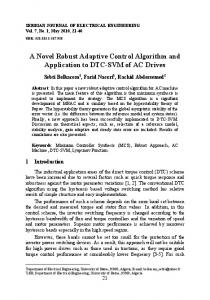
Continuous Stirred Tank Reactor (CSTR) A stirred tank Fig1 is the most fundamental of mixers and many common mixers from the Brabender mixer used in lab to a cup of coffee with a spoon can be considered a stirred tank under some set of approximation. Mixing in a stirred tank is complicated and not well described although the use of dimensionless numbers and comparison with literature accounts can lead to some predictive capabilities. Often stirred tanks are used as industrial reactors where a chemical component of a flow stream resides for some time in the tank and then proceeds on to other steps in a chemical process. The residence time distribution becomes a measure of the extent of a chemical reaction in this situation. For mixing one can sometimes assume a constant rate of strain in the stirred tank and the residence time distribution can then be used under this approximation, as a measure of the extent of mixing. Dead zones in a stirred tank for high viscosity fluids should be very familiar to anyone who has worked in a kitchen mixing dough with a hand mixer. Fluid motion in a stirred tank is confined to the immediate region of the mixer blades for high viscosity fluids (Al-Naemi and Abdalla, 2004). Table 1: Design Parameters and Operating Conditions of the CSTR Item symbol Value Dimension Length
L
2.00
m
Diameter
D
1.85
m
Feed Temperature
Tf
210.00
Feed Pressure
PR
1.03
bar
Total Molar flow Rate
FR
100.00
mole.min-1
Feed Concentration
CI
6.90
mole.dm-3
o
C
Residual Fluid Catalytic Cracking (RFCC) Reactor Vessel Fluid catalytic reactor vessel comprising: at its upper end a single centrally positioned primary cyclone having a gas-solids inlet fluidly connected to the downstream iterations") that never attempt to iterate any optimization problem to convergence, but instead only one iteration
NUJES Al Neelain University Journal of Engineering Sciences, VOL 1, No. 1, December 2013 Table 2: Design Parameters Conditions of the RFCC
Figure1: The Continuous Stirred Tank Reactor (CSTR) end of a fluid catalytic riser, which riser is positioned externally from a fluid catalytic reactor vessel; said primary cyclone further provided with a gas outlet conduit at its upper end fluidly connected to one or more secondary cyclone separators, which secondary cyclone separators are positioned in the space between the centrally positioned primary cyclone and the wall of the reactor vessel and which secondary cyclones have means to discharge solids to the lower end of the reactor vessel and means to discharge a gaseous stream poor in solids to a gas outlet of the reactor vessel; said primary cyclone further provided with a primary stripping zone at its lower end and means to discharge pre-stripped solids from the primary cyclone to the lower end of the reactor vessel; and wherein the reactor vessel further comprises at the lower end of reactor vessel a secondary stripping zone is and means to discharge stripped solids from the reactor vessel.
Figure 2: Residual Fluid Catalytic Cracking Unit against any safety factors that otherwise must be applied
35
and
Operating
Item
Symbo l
Valu e
Dimensio n
Length
L
3.8
m
Diameter
D
2.5
m
Feed Temperature
Tf
210
o
Feed Pressure
PR
0.2
MPa
Total Molar flow Rate
FR
225
Ton/hr
Feed Concentratio n
CI
NA
NA
C
Table 2 show the design parameters and operating conditions of the RFCC used in this simulation.
Mathematical Models A model of a reaction process is a set of data and equations that are believed to represent the performance of a specific vessel configuration (mixed, plug flow, laminar, and dispersed, and so on). The equations include the stoichiometric relations, rate equations, heat and material balances, and auxiliary relations such as those of mass transfer, pressure variation, contacting efficiency, residence time distribution, and so on. The data describe physical and thermodynamic properties and, in the ultimate analysis, economic factors. Correlations of heat and mass-transfer rates are fairly well developed and can be incorporated in models of a reaction process, but the chemical rate data must be determined individually. The most useful rate data are at constant temperature, under conditions where external mass transfer resistance has been avoided, and with small particles with complete catalyst effectiveness. Equipment for obtaining such data is now widely used, especially for reactions with solid catalysts, and it is virtually essential for serious work. Simpler equipment gives data that are more difficult to interpret but may be adequate for exploratory work. Once fundamental data have been obtained, the goal is to develop a mathematical model of the process and to utilize it to explore such possibilities as product selectivity, start-up and shut-down behavior, vessel configuration, temperature, pressure, and conversion profiles, and so on. How complete a model has to be is -Coolant Temperature. The outputs were:
36
NUJES Al Neelain University Journal of Engineering Sciences, VOL 1, No. 1, December 2013
an open question. Very elaborate ones are justifiable and have been developed only for certain widely practiced and large-scale processes or for processes where operating conditions are especially critical. The only policy to follow is to balance the cost of development of the model to a final process design. Engineers constantly use heat and material balances without perhaps realizing, like Moliere’s Bourgeois that they are modeling mathematically. The simplest models may be adequate for broad discrimination between alternatives (Abdalla and Elnashaie, 1995a, 1995b).
-Product Temperature. -Residual Concentration. The simulation program of the MATLAB Simulink was then run. The results obtained were then compared with industrial ones.
α J = AB ( K BD ) JB assume α J = 1
Toolbox Graphic User Interphase GUI
Results and Discussion
Based on the model formulation section of chapter 4, and the design parameters of the CSTR and the RFCC as well as the industrial operating conditions of the RFCC of the Khartoum Refinery (KRC, Sudan); the MPC inter phase of the MATLAB was used to simulate the industrial Material Balance of Bubble Phase cases selected. The results of controlling the two −α j h N JB = QB [( N JD / QD ) − {( N JD / QD ) − ( N JB / QB )}e ] processes selected are explained below. Figure 3 shows the design of CSTR and the RFCC in the MATLAB Graphic User Interphase (GUI) work space.
Where Nj: Molar flow rate of component j (kmol/s) Q : Volumetric rate (m٣ /s) h:Rector table height (m) A: cross-sectional area (m2) (KBD)JB: Interphone mass transform coefficient between bubble and dense phase based on bubble volume (I/S). Subscripts: B- Bubble phase D- Dense phase Energy Balance of Bubble Phase:
TB = TD − (TD − TBf )e − Bh
β=
AB ( H BD ) B PG C PG QB
assume β = 1.0 Where: T = Temperature (K) (HBD)B: inter phase heat transfer coefficient between bubble and dense phase based on bubble phase volume (Kg/m3/s/K).
Linking the Model with Self-tuning The model equations provided above were used for designing the different Graphic User Interfaces (GUI) used in this simulation. The MATLAB help file provided the procedure steps on the formulation and design of the GUI (MATLAB User Guide, 2004). The designed GUI was then provided with the model equations and the industrial Parameters obtained from the KRC. The application was made on two refinery units mainly the Atmospheric Distillation Unit (ADU) and the Residual Fluid Cracking Unit (RFCC) by making different manipulations to the inputs, namely temperature and feed concentration. The inputs were: -Feed Concentration. -Feed Temperature.
Figure3: MPC of CSTR Operating temperatures and molar feed rates concentrations of the CSTR and the RFCC were selected and introduced to the GUI as shown in the Figure 3. The design parameters and the operating conditions of the CSTR and the RFCC are shown in Tables 1 and 2. The results of the simulation using the GUI are shown below. The results of figures 4 and 5 show the results of using the non-linearized design equations of the CSTR and the RFCC.
Result of Continuous Stirred Tank Reactor [CSTR] Figure 4 shows the step changes of the three operating conditions of the CSTR. The results showed very good response with operating conditions. Since the nonlinearity of the CSTR is not stiff compared to the RFCC the step changes only affected the feed and output concentrations; while the boiler and the reactor temperatures are not affected. Also if the CSTR is assumed isothermal the temperature changes effects will be negligible. Since the RFCC is more rigorous and multiphase system;
NUJES Al Neelain University Journal of Engineering Sciences, VOL 1, No. 1, December 2013
37
the design equations and the operating conditions are highly nonlinear. The results of figure 5 clearly say the nonlinearity of the equations is of noticeable effect on the step changes of the system. This was shown on the changes took places of the three parameters investigated.
Figure4: Results of Continuous Stirred Tank Reactor before linearization.
Results of the Residual Fluid Catalytic Cracking [RFCC] Figure 6: Results of the MPC design input delay 0 for the input to RFCC
Figure5: Results of the Residual Fluid Catalytic Cracking (RFCC) Unit before linearization. The results of Figure 5 clearly illustrate that the nonlinearity of the equations are of noticeable effect on the step changes of the system. This was shown when
Figure 7: Results of MPC design output delay 0 for the output of the RFCC. The results of Figure 5 suggested that a linearization scheme is a must in these industrial cases. Since the MPC of the employed MATLAB has the tools to handle this situation; a linearization scheme was used and the results
38
NUJES Al Neelain University Journal of Engineering Sciences, VOL 1, No. 1, December 2013
are shown in Figures 6 and 7. The results showed that the three parameters investigated were manipulated. linearization of the three input parameters promptly affected the industrial outputs. The results of employing the Model Predictive Control of the MATLAB clearly explain the idea of self-tuning control system to an industrial case like the Residual Catalytic Cracker [RFCC] of crude oil refining process. This idea is not new for industrial application but the approach taken in this study was a successful trial when the MPC is used coupled with the self-tuning adaptive control strategy (Birchfield, 1996; Kothare, et.al., 1996; Lee and Yu, 1997; Lee, et.al., 1992).
Conclusions Many simulations, digital and analog, were performed in which self-tuning regulators were made to follow set points by use of Wittenmark’s method of cascading integrator. The technique was shown to be powerful and practical. A modification to the technique was proposed and demonstrated, namely the cascading of a PI block with a drifting type 1 system under self-tuning control. A servo self-tuning scheme was proposed, in which the set point was following and regulation parts of the selftuner were separated. Several examples of servo selftuners were presented. The servo self-tuning scheme was shown to produce interesting identification results as a by-product of self-tuning control. Some servo selftuning schemes were shown to be equivalent to the schemes of Clarke and Astrőm. These schemes were browed and implemented using the Model Predictive Control (MPC) of the MATLAB GUI work space toolboxes. The project’s first main achievement in the practical features of self-tuning control was the definition of a simple but effective limit reflection and integral windup protection technique. Extensive studies were made into the problems of initialization of self-tuners and results and guidelines have been presented. Two methods of handover of control have been presented, namely handover by prior simulation, and handover by “open loop” tuning to the system under fixed-term digital control. The point has been made that self-tuned control laws can be fixed as conventional digital control laws. It has been asserted that self-tuning can be used as an online controller design tool, to good effect. The control problems of some non-linear systems were looked at, and some distinctions drawn to classify those nonlinearity with which self-tuning can and cannot cope. The application of these schemes when coupled with the MPC and the model and design equations of the industrial equipment under investigation showed clear and progressive success on using these type of controlling systems for industrial purposes.
References Abdalla, B. K. and S.S.E.H. Elnashaie, 'A Modified Model for the Fluidized Bed Reactor for the Catalytic Steam Reforming of Methane'. J. King Saud Univ. 7, [Engng. Sci.]. (Special Issue), 271-282, (1995). Abdalla, B. K. and S.S.E.H. Elnashaie, 'Fluidized Bed Reactors without and with Selective Membranes for the Catalytic Dehydrogenation of Ethylbenzene to Styrene'. J. Of Membrane Sci., 101, 31-35, (1995). Al-Naemi, M. and Abdalla, B. K., 2004, “Predictive Control of Unknown Nonlinear Systems”, 12th Mediterranean Conference on Control and Automation (MED' 04) Turkey. Birchfield, G. S., 1996, “Trends in Optimization and Advanced Process Control in the Refinery Industry”, Chemical Process Control V, Tahoe City, CA. Borrison U, and Syding, 1976, “ Self-Tuning Control of an Ore Crusher”,Automatica 12 pp. 1-7. Cegrell T. and Hedqvist T., 1975 “ Successful Adaptive Control of Paper Machines”, Automatica 11 pp. 53-59. Csaki F., Keviczky L.K.,Hetthessy J., Hilger M.and Kolostori J., 1978,” Simultaneous Adaptive Control of Chemical Composition, Fineness and Maximum Quantity of Ground Materials at a Closed Circuit Ball Mill”, Proc. IFAC 7th World Congress, Helsinki, Finland. Clarke D.W., Dyer D.A.J., Hastings-James R.,Ashton R.P. and Emery J.B., 1973, “ Identification and Control of a Pilot-Scale Boiling Rig”, Proc. IFAC 3rd Symposium on Identification and System Parameter Estimation, The Hague/Delft, Holland. Dumont G., 1977, “Control and Optimization of Titanium Dioxide Klns”, Ph.D. Thesis, Dept.of Electrical Eng., McGill University. Dumont G.A. and Belanger P.R., 1978,” Self-Tuning Control of a Titanium Dioxide Kiln”, IEEE Trans. Auto. Control AC-23 pp 532-538. Horn J.E., 1978, “Feasibility Study of the Application of Self –Tuning Controllers to Chemical Batch Reactors” OUEL Report 1248/1978, Oxford Univ.,U.K. Jensen L. and Hansel R., 1974, “Computer Control of an Enthalpy Exchanger”, Report 7417, Div.of Aut. Control, Lund Inst. Tech., Sweden. Kallstrom C.G., 1974, “The Sea Scout Experiments”, Report 7407 (c), Div. Aut. Control, Lund Inst. Tech., Sweden. Kallstrom C.G., Aström K.J., Throell N.E., Eriksson, and Sten L., 1977,” Adaptive Autopilots for Steering of Large Tankers”, Lund Report no. LUTFD2/(TFRT3145)/1-66/(1977), Lund. Inst. Tech., Sweden. Kallstrom C.G. Aström K.J., Thorell N.E., Eriksson J. and Sten L., 1978, “Adaptive Autopilots for Lare Tankers”, Proc. IFAC 7th World Congress, Helsinki, Finland. Kalman R.E., 1958, “ Design of a Self-Optimizing Control System”, Trans. ASME.
NUJES Al Neelain University Journal of Engineering Sciences, VOL 1, No. 1, December 2013 Keviczky L., Hetthessy J., Hilger M. and Kolostori J., 1978, “ Self-Tuning Adaptive Control of Cement Raw Material Blending”, Automatica, 14 pp 525-532. Kothare,M .V,V., Balakrishman,and M.Morari,1996”Robust constained model predictive control using linear matrix inequalities”,Automatica,32,10,1361-1379 Lee, J. H., and Z Yu, 1997 ”Worst-Case Formulation of Model Predictive Control for System with Bounded Parameters”, Automatica,33,763-781. Lee, J. H., M. S. Gelormino, and M. Morari, 1992, “Model Predictive Control for Multi-Rate Sampled Data Systems”, Int. J. Control, 55,153-191. Model Predictive Control Toolbox 2, Develop internal model-based controllers for constrained multivariable processes, by the MathWorks Inc. MATLAB, 2004. Morris A.J., Fenton T.F. and Nazer Y.,1977, “ Application of Self-Tuning Regulators to the Control of Chemical Processes”, IFAC Congress on Digital Computer Applications to Process Control, The Hague, Holland.
39
Morris A.J., Nazer Y. and Chisholm K.,1979, “ Single and Multivariable Self Tuning Microprocessor-Based Regulators”, 3rd IEE Conference on Trends in On Line Computer Control Systems, Sheffield, UK, ( IEEE Conference publ. 172). Sastry V.A., Seborg D.E. and Wood R.K., 1977, “ Self – Tuning Regulator Applied t a Binary Distillation Column”, Automatica, 13 pp 417-424. Wittenmark B., 1975, “Stochastic Adaptive Control Methods- A Survey” , Int. J. Control, 21, pp 705-730. Wouters W.R.E., 1974, “Parameter Adaptive Regulators, Control for Stochastic SISO Systems, Theory and Applications”, Proc. IFAC Symposium on Stochastic Control, Budapest. Wouters W.R.E., 1977, “Adaptive Pole Placement for Linear Stochastic Systems with Unknown Parameters” Proc. IEEE Conference on Decision and Control, New Orleans, USA.