semi-definite programming approach to sensor network node ...

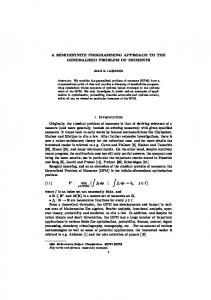
SEMI-DEFINITE PROGRAMMING APPROACH TO SENSOR NETWORK NODE LOCALIZATION WITH ANCHOR POSITION UNCERTAINTY Kenneth W. K. Lui∗ , W.-K. Ma† , H. C. So∗ and Frankie K. W. Chan ∗ ∗

Department of Electronic Engineering, City University of Hong Kong Tat Chee Avenue, Kowloon, Hong Kong † Department of Electronic Engineering, The Chinese University of Hong Kong Shatin, N.T., Hong Kong ABSTRACT The problem of node localization in a wireless sensor network (WSN) with the use of the incomplete and noisy distance measurements between nodes as well as anchor position information is currently an an important yet challenging research topic. Most WSN localization studies at present have assumed that the anchor positions are perfectly known which is not valid in the underwater and underground scenarios. In this paper, semi-definite programming (SDP) algorithms are devised for finding the localizations of unknown-position nodes in the presence of anchor position uncertainty. Computer simulations are included to contrast the performance of the proposed algorithms with the conventional SDP method and Cram´er-Rao lower bound. Index Terms— sensor networks, node localization, range measurements, semi-definite programming I. INTRODUCTION A wireless sensor network (WSN) consists of a number of small spatially distributed wireless devices or devices which can perform computation, communication, sensing and control tasks. They are able to take environmental measurements, such as temperature, light, sound pressure and humidity for a wide range of monitoring and control applications in the military, environmental, health and commercial aspects [5]– [8]. Due to the mostly arbitrary node deployment, the sensor locations are often unknown. As a result, determining the physical positions of the sensor nodes is an important problem in the WSNs. In this paper we consider determining the absolute positions of sensor nodes in a network given incomplete and noisy pairwise distance measurements [5]– [8], which are constructed from the received signal strength or time-of-arrival information acquired by the sensors during communications with their neighbors. A standard assumption is that the positions of some nodes, called anchors, are known exactly. In the presence of Gaussian disturbance, the maximum-likelihood estimator (MLE) for WSN location estimation is devised in [5] which corresponds to a multi-variable non-linear optimization problem and is hard to implement in practice. The MLE can be realized by stochastic optimization methods such as genetic algorithm and simulated annealing [6] but they involve intensive computations with no guarantee of attaining the global optimum point. Alternatively, it is possible to relax the MLE formulation to a semi-definite programming (SDP) problem [7]– [8] in order to provide a high-fidelity approximate solution that can be obtained in a globally optimum fashion with reduced computational efforts. However, most WSN localization studies [5]– [8] concentrate on the case when the anchor positions are perfectly known. In this paper, we devise novel SDP algorithms for node localization using noisy pairwise distance measurements

978-1-4244-2354-5/09/$25.00 ©2009 IEEE

2245

in the presence of this uncertainty. A representative application scenario is an underwater WSN [9] where there are three types of nodes, namely, surface buoys, anchors and unknown-position nodes. Surface buoys drift on the water surface and they can get their absolute locations from global positioning system (GPS) or by other means. The anchors estimate their positions through communications with the buoys and this implies the presence of anchor position uncertainty. As in conventional WSNs, the ordinary nodes communicate with each other as well as the anchors to estimate their positions as they do not have wireless connections with the buoys. Note that even GPS-based positioning cannot give error-free location solutions as well. It is noteworthy that [10] has recently studied the impact of anchor position uncertainty in node localization but the suggested convex optimization approach is not derived from the MLE. The rest of the paper is organized as follows. Assuming that both the distance errors and anchor position errors are Gaussian distributed, the MLE for node localization with anchor location uncertainty is first developed in Section II. In addition, further approximation on the developed algorithm based on the edgebased semi-definite programming (ESDP) [11] which allows a more computationally efficient realization is suggested. The proposed WSN positioning algorithms are evaluated by comparing with the standard SDP approach as well as Cram´er-Rao lower bound (CRLB) in Section III. Finally, conclusions are drawn in Section IV. II. PROPOSED METHOD To start with, we would like to introduce the notations used in this paper. Bold upper case symbols denote matrices and bold lower case symbols denote vectors. We use {·}o to represent the true value ˆ The 0m×n ∈ Rm×n while its variable is {·} and its estimate is {·}. and 0n ∈ Rn×n are zero matrices and In ∈ Rn×n is the identity matrix. For two symmetric matrices A and B, A  B is equal to A − B  0 which indicates that A − B is positive semi-definite. Trace operator of matrix A is denoted by Tr(A). The T and −1 denote matrix transpose and inverse operators, respectively, and x2 represents the 2-norm of a vector x. Consider a network of m sensors in a two-dimensional space. Let xoi = [xoi , yio ]T , i = 1, 2, · · · , m, be the true position of the ith node. Without loss of generality, we assume that the first k of them, xo1 , xo2 , · · · , xok , are the anchor positions while xok+1 , xok+2 , · · · , xom , correspond to the unknown-position sensors. For absolute positioning, it required that k ≥ 3. In this Section, we consider that there is position uncertainty in the anchor information and our task is to find better estimates of the k anchor positions as well as the n = (m − k) unknownsensor locations, or to estimate Xo = [xo1 , xo2 , · · · , xom ] ∈ R2×m . By further relaxing the constraints in the proposed SDP algorithm,

ICASSP 2009

we then provide its computationally efficient approximation using the ESDP.

γij and X is 2 = xi − xj 2 = yii + yjj − yij − yji , γij = rij

i = k + 1, k + 2, · · · , m,

II-A. SDP algorithm development o , i, j = 1, 2, · · · , m, be the distance from the ith node Denote rij to jth node. In the absence of measurement error, a simple relation between them is q o o = rji = (xoi − xoj )2 + (y o − yjo )2 rij (1) = xoi − xoj 2 , i, j = 1, 2, . . . , m

In the presence of distance errors and anchor position errors, our o + eij , i = j = 1, 2, . . . , m, and ai = observations are dij = rij o xi + ui , i = 1, 2, . . . , k. Each ai ∈ R2×1 represents an erroneous anchor position. The disturbances eij and ui ∈ R2×1 are assumed to be independent zero-mean Gaussian processes with variances and 2 and Φi ∈ R2×2 , respectively. Note that we covariance matrices σij only have an incomplete set of {dij } due to limited communication ranges between nodes. Without loss of generality, we assume that all the distance measurements between {ai } are not available. Let X = [x1 , x2 , · · · , xm ] be the variable matrix for Xo and A = [a1 , a2 , · · ·, ak ]. Under Gaussian disturbance assumption, the MLE for Xo is achieved by maximization of the probability of p({dij }, A|X). As {eij } and {ui } are independent, the probability can be expressed as p({dij }, A|X) = p({dij }|X)

k Y

Furthermore, we denote Ξi = xi xTi . The second last term of (5) will become k X

δij |dij − xi − xj 2 |2 2 σ ij i,j=k+1

(3)

i>j

+

k X

(ai − xi )T Φ−1 i (ai − xi )

i=1

where δij = 1 if the distance measurement is available and 0 otherwise. The first and second terms of (3) correspond to the distances between the anchors and unknown-position sensors, and distances among the unknown-position sensors, respectively, while the last term addresses the anchor position uncertainty. To simplify the expression, we define gij : ( 2 δij /2σij , i > k and j > k gij = (4) 2 δij /σij , otherwise Expanding the objective function in (3) and dropping the irrelevant terms yields an equivalent cost function: m m X X

ˆ ˜ gij xi − xj 22 − 2dij xi − xj 2

i=k+1 j=1

+

k X

(5) xTi Φ−1 i xi

−

m m X X

X,Y,{Ξi },{γij },{rij } i=k+1 j=1

2aTi Φ−1 i xi

i=1

In order to form a tight constraint in the later relaxation procedure, we introduce two dummy variables γij and rij for the first term and second term of (5), respectively. Then a constraint which relates

2246

(8)

+

gij [γij − 2dij rij ]

k h i X T −1 Tr(Φ−1 i Ξi ) − 2ai Φi xi i=1

γij = yii + yjj − yij − yji

(9)

2 rij = γij ,

i = k + 1, k + 2, · · · , m,

i=k+1 m X

+

Tr(Φ−1 i Ξi )

i=1

min

Tr(Ξi ) = yii ,

Maximizing (2) is equivalent to the nonlinear least squares (NLS) problem: min

k X

For the sake of establishing a relationship between Ξi and yii , we utilize Ξi to introduce Tr(Ξi ) = xTi xi = yii , i = 1, 2, · · · , k as a further constraint. With the use of all developed constraints, the MLE of (3) is equivalent to the following formulation:

i=1

X∈R2×m

xTi Φ−1 i xi =

i=1

(2)

m k X X δij |dij − xi − xj 2 |2 2 σ ij j=1

(6)

where yij = xTi xj is the (i, j) entry of the matrix Y which is defined as – » T X X XT (7) Y := X I2

s.t. p(ai |xi )

j = 1, 2, · · · , m

Ξi = xi xTi , » T X X Y= X

j = 1, 2, · · · , m

i = 1, 2, · · · , k i = 1, 2, · · · , k –

XT I2

We now relax (9) to a convex optimization problem as follows. 2 = γij in (9) will be replaced by the inequality The equality rij 2 rij ≤ γij to meet the convex specification. In fact, rij and γij will increase and decrease in the minimization, respectively, a tight constraint is automatically achieved, and thus the inequality constraint will be forced to an equality. In addition, performing semi-definite relaxation on (7) and Ξi = xi xTi , the MLE of (9) is approximated as a convex optimization problem: m m X X

min

X,Y,{Ξi },{γij },{rij } i=k+1 j=1

+

gij [γij − 2dij rij ]

k h i X T −1 Tr(Φ−1 i Ξi ) − 2ai Φi xi

(10)

i=1

s.t.

γij = yii + yjj − yij − yji 2 rij

(11)

≤ γij , i = k + 1, k + 2, · · · , m,

(12) j = 1, 2, · · · , m

i = 1, 2, · · · , k Tr(Ξi ) = yii , – » Ξi x i  03 , i = 1, 2, · · · , k xTi 1

(13)

Y  0m+2

(15)

i = 1, 2, · · · , m xi = [yi m+1 , yi m+2 ]T , – » ym+1 m+1 ym+1 m+2 = I2 ym+2 m+1 ym+2 m+2

(16)

(14)

(17)

where all the constraints are tight except (14) and (15) which im-

pose rank relaxation on the matrices. In the optimization literature, there are readily available solvers for finding the globally optimum SDP solution for (10)−(17), such as S E D U M I [12] and SDPT3 [13]-[14]. Although the centralized approach is studied in this work, the proposed method can be easily extended to the decentralized scenario by dividing the WSN into clusters of smaller sub-networks [7] – [8]. II-B. Edge-based SDP As the arithmetic operation complexity of the SDP is at least O(m3 ) [11], it is desirable to have a more computationally efficient solution particularly when the network size is large. One recent SDP development which can achieve efficient and accurate estimation while retaining its key theoretical property is to relax the single semi-definite matrix cone into a set of small-size cones, and this is known as ESDP relaxation [11]. The ESDP version of our proposed algorithm is simply achieved by replacing the single (m + 2)dimensional matrix cone Y in (17) with at most m(m − 1)/2 4-dimensional matrix cones: 3 2 yii yij xTi T 4 yji yjj xj 5  04 , (18) xi xj I2 i, j = 1, 2, · · · m,

i > j,

and ESDP methods, we see that the improvement over the standard one increases with the anchor position error. The computation times and MSEs of the proposed SDP and ESDP algorithms are studied for different number of nodes, and the results are tabulated in Table I. The number of anchors is fixed at k = 8 with the same positions as in the above tests. The unknown-position nodes are placed inside the 40m × 40m area where the communication range is governed by 0.3(40 × 40)/m and σd2 = −20 dBm2 is assigned. It is observed that for a larger WSN, the EDSP scheme is much more computationally efficient than the SDP method at the expense of higher MSEs. IV. CONCLUSION Assuming Gaussian distributed disturbances, the nonconvex maximum likelihood estimation for sensor network node localization in the presence of anchor position uncertainty has been approximated to a convex optimization problems using the semidefinite programming (SDP) relaxation technique. It is shown that when the anchor positions are of errors, the proposed SDP and its edge-based variant algorithms can give very accurate node localization performance.

δij = 1

ACKNOWLEDGEMENT

That is, (10)−(17) and (18) correspond to the ESDP relaxation algorithm for node localization in the presence of anchor position uncertainty.

The work described in this paper was supported by a grant from the Research Grants Council of the Hong Kong Special Administrative Region, China (Project No. CityU 119606).

III. SIMULATION RESULTS

V. REFERENCES

Computer simulation has been conducted to evaluate the performance of the proposed SDP node positioning approach in the presence of anchor position error. Comparison with the standard SDP algorithm based on MLE [7] which assumes perfect anchor position information and the corresponding CRLB is also made. We utilize the MATLAB toolbox YALMIP [15] to realize all SDP algorithms where the solver SDPT3 [13]-[14] is employed. For the mean square error (MSE) performance evaluation, only the estimates for the unknown-position nodes are involved in the computation as the standard algorithm cannot fine tune the anchor positions, and all the results are based on averages of 500 independent runs. The range errors {eij } are zero-mean white o }, which means Gaussian variables with standard deviations {σd rij that a larger range will correspond to a larger variance, and we scale the values of σd to obtain different noisy conditions. We first consider a WSN of 18 sensors with 8 of them are anchors and its configuration is depicted in Figure 1. In this WSN geometry, nodes are partially connected and the maximum communication range between nodes is set to be 25m which corresponds to an average node degree [16] of 8.67. In the first experiment, we investigate the performance of the SDP algorithms in the presence of anchor position uncertainty. All anchor position covariance matrices are assigned as Φi = κ2i I2 with κ2i = −10 dBm2 for all i. Figure 2 shows the MSEs of the position estimates versus σd2 we see the superiority of the proposed SDP and ESDP methods over the standard one particularly for smaller noise conditions, although the two SDP algorithms give nearly the same performance when σd2 ≥ −30 dBm2 . It is also observed that the performance of our SDP method is close to the CRLB while the ESDP version only degrades the tighter SDP scheme by less than 0.5 dBm2 . The MSE results versus κ2i at σd2 = −50 dBm2 are plotted in Figure 3. Apart from higher estimation performance of the proposed SDP

[1] I.F. Akyildiz, W. Su, Y. Sankarasubramaniam and E. Cayirci, “A survey on sensor networks,” IEEE Communications Magazine, pp.102-114, Aug. 2002 [2] M. Ilyas and I. Mahgoub, Handbook of Sensor Networks: Compact Wireless and Wired Sensing Systems, London: CRC Press, 2005 [3] A. Swami, Q. Zhao, Y.-W. Hong and L. Tong, Wireless Sensor Networks: Signal Processing and Communications Perspectives, NJ: Wiley, 2007 [4] N. Patwari, J.N. Ash, S. Kyperountas, A.O. Hero, III, R.L. Moses and N.S. Correal, “Locating the nodes: cooperative localization in wireless sensor networks,” IEEE Signal Processing Magazine, pp.54-69, July 2005 [5] N. Patwari, A.O. Hero, III, M. Perkins, N.S. Correal and R.J. O’Dea, “Relative location estimation in wireless sensor networks,” IEEE Trans. Signal Processing, vol.51, vol.8, pp.21372148, Aug. 2003 [6] A.A. Kannan, G. Mao and Branka Vucetic, “Simulated annealing based localization in wireless sensor network,” Proc. IEEE Conf. Local Computer Networks, pp.513-514, 2005, Washington, USA [7] P. Biswas, T.-C. Liang, T.-C. Wang and Y. Ye, “Semidefinite programming based algorithms for sensor network localization,” ACM Trans. Sensor Networks, vol.2, no.2, pp.188-220, May 2006 [8] P. Biswas, T.-C. Liang, K.-C. Toh, Y. Ye and T.-C. Wang, “Semidefinite programming approaches for sensor network localization with noisy distance measurements,” IEEE Tran. Auto. Sci. and Eng., vol.3, no.4, pp.360-371, Oct. 2006 [9] Z. Zhou, J.-H. Cui and S. Zhou, “Localization for large-scale underwater sensor networks,” NETWORKING 2007, LNCS 4479, pp.108-119. 2007

2247

k+n 8+2 8+4 8+8 8+16 8+32

Range (m) 48 40 30 20 12

Connectivity 8.5216 8.6007 8.8230 8.6188 6.6020

SDP time (s) 0.2802 0.3345 0.4905 1.2346 5.0113

ESDP time (s) 0.3367 0.4500 0.6282 0.9322 1.5199

SDP MSE (m 2 ) 2.4935 1.6548 1.2497 1.0707 2.3573

ESDP MSE (m2 ) 2.4929 1.6622 1.2864 1.2013 3.5761

TABLE I: Computational time and mean square error comparison for proposed SDP and ESDP schemes

2 0 2

Mean square position error ( dBm )

[10] S. Srirangarajan, A.H. Tewfik and Z.-Q. Luo, “Distributed sensor network localization with inaccurate anchor positions and noisy distance information,” Prof. ICASSP 2007, vol.III, pp.521-524, Honolulu, Hawaii, USA, Apr. 2007 [11] Z. Wang, S. Zheng, Y. Ye and S. Boyd, “Further relaxations of the SDP approach to sensor network localization,” SIAM J. Optimization, vol. 19, no.2, pp.655–673, Jul. 2008 [12] J.F. Sturm, “Using SeDuMi 1.02, a M ATLAB toolbox for optimization over symmetric cones,” Optim. Methods Softw., vol. 11–12, pp.625–653, 1999, http://sedumi. mcmaster.ca/ [13] K.C. Toh, M.J. Todd and R.H. Tutuncu, “SDPT3 — a M ATLAB software package for semidefinite programming,” Optimization Methods and Software, vol.11, pp.545-581, 1999 [14] R.H. Tutuncu, K.C. Toh and M.J. Todd, “Solving semidefinitequadratic-linear programs using SDPT3,” Mathematical Programming Ser. B, vol.95, pp.189-217, 2003, http://www. math.nus.edu.sg/˜mattohkc/sdpt3.html [15] J. L¨ofberg, “YALMIP : a toolbox for modeling and optimization in MATLAB,” Proc. Int. Symp. CACSD, pp.284-289, Taipei, Taiwan, Sept. 2004 [16] K. Langendoen and N. Reijers, “Distributed localization in wireless sensor networks: a quantitative comparison,” Computer Networks, vol.43, pp.499-518, 2003

−2 −4 −6 −8 −10 −12

standard SDP proposed SDP proposed ESDP CRLB

−14 −16 −50

−45

−40

−35 2 d

−30

−25

−20

2

σ ( dBm )

Fig. 2. Mean square position error versus σd2 in the presence of anchor position uncertainty

20 15 10 −12

0

−14

−5

2

Mean square position error ( dBm )

y (m)

5

−10 −15 −20 sensor −25

−20

−15

−10

−5

0 x (m)

anchor 5

10

15

20

Fig. 1. Geometry of sensor network

−16 −18 −20 −22 −24 −26

standard SDP proposed SDP proposed ESDP CRLB

−28 −30 −30

−25

−20

−15

−10

κ2 ( dBm2 ) i

Fig. 3. Mean square position error versus κ2i at σd2 =−50dB

2248