Sensorless Peak Power Point Tracking System for Small Scale Wind Turbine Generators Md. Wasi Uddin, Md. Yiasin Sumon, Rajib Goswami, Md. Rahimul Hasan Asif and K. M. Rahman Department of Electrical and Electronic Engineering Bangladesh University of Engineering and Technology, Dhaka-1000 E-mail:
[email protected]
Abstract: This paper describes a small wind energy conversion system with an application of a simple and efficient peak power tracking algorithm. This real time approach enables the controller to extract the maximum available power from the wind and use this power to charge a sealed lead-acid battery (SLA). Calculating the differential power from the power-frequency curve tracking of the inflection point is possible and that leads to the maximum power point. The concept of the system has been analyzed and simulated using a permanent magnet synchronous generator (PMSG) directly coupled with a wind turbine in Simulink.
1. Introduction Limitation of available energy sources worldwide and the environmental pollution caused by fossil fuel used for electricity generation has given the renewable energy sources supreme importance. The remote areas where power grid connection is not possible, renewable energy sources like wind energy might be a good alternative. The maximum power of a wind turbine depends on the corresponding wind speed. Generally the wind turbine is surrounded by several anemometers to measure wind speed which eventually increases cost and complexity of a system. But recently some methods are developed where mechanical sensors are not required. These approaches can be classified as real time and non-real time approaches. In non-real time approaches, the wind speed is estimated in some ways like ANN (artificial neural network), fuzzy logic or using lookup tables. After finding wind speed, the corresponding maximum power can be drawn. Real time approach means runtime Peak Power Point Tracking (PPPT) using any defined algorithm. Most of the research works regarding the real time approach have been on slope calculation basis. In this paper, sensor-less slope calculation based PPPT algorithm is introduced which is simple, efficient and fast. For a specific wind speed power (p) versus generator speed (f) curve of a wind energy system is an inverse Ushaped non-linear curve having a single maximum point. For efficient power extraction, System Operating Point (SOP) should be at Peak Power Point (PPP) of the curve. But in real world wind speed doesn’t remain constant all the time. These wind speeds introduce different wind curves each having individual PPP. Our PPPT algorithm
finds a way to the runtime PPP by changing the movement of SOP. Measuring different powers and frequencies the runtime slopes are calculated which are used to find the inflection point and eventually the PPP. The algorithm is experimentally verified in a simulated system. The Block diagram of the simulated system is shown in Fig. 1. The controller acquires the required input parameters from the load and generator side and with PPPT algorithm Pulse Width Modulated Waveform (PWM) is adjusted by varying the duty cycle and applied to the DC converter circuit to control the power demand. Eventually it attains the SOP at PPP.
Fig. 1 Block diagram for the maximum power tracking system
2. Maximum power tracking 2.1
Turbine characteristics
Power of a wind turbine depends on various parameters e.g. power coefficient, wind speed, tip speed ratio etc. A Wind turbine can be characterized by the following equations. 1 P = ρAV 3C p ω m 2 Cp(λ , β ) = 0.5176(
1
λi λ=
=
116
λi
(1) − 0.4β − 5)e
1 0.035 − 1 + 0.08β β 3 + 1
V
ω
W r
ω
Where, P = mechanical input power
m
−
21
λi − 0.0068λ
(2) (3) (4)
ρ = density of air, (1.205 kg/m3 assumed for simulation) A = area swept by blades, (1.7 m simulation) V = wind speed
2
assumed for
ω
C p = turbine power coefficient
β = blade pitch angle (assuming 00) r = turbine blade radius λ = tip speed ratio (TSR)
Wω = generator speed 0.5
0.48
0.45 0.4 0.35
Cp
0.3 0.25 0.2 0.15 0.1 0.05 0
8.1 0
2
4
6
8
10
12
λ
Fig. 2 CP versus λ curve
In Fig. 2 C p versus λ curve is plotted using equation [2]. The maximum value of C p =0.48, when λ =8.1. For different wind speeds the value of maximum power coefficient and tip speed ratio should be around these values
2.2
increased to increase the loading in such a manner that the increment in duty is greater than the previous increment by a value ‘k’(increment= previous_increment+k). Here ‘k’ is an adjusted constant which depends on the turbine characteristics and wind speed ranges. In this way, up to the point of inflection the rate of loading is increased linearly. (In a function with maxima, the differential slope is negative at one side and positive at the other. The inflection point is in the middle of them and there the differential slope is zero. As this point is near the maximum point it is used to achieve the maximum power point quickly.) Step 3: After crossing the inflection point the rate of increment is kept constant. Through this constant increase when case 2 is matched at point P3 the SOP reaches PPP. Step 4: While operating at point P3 if the wind speed is changed from v1 to v3 (Fig. 3), the PPP is changed for this new wind curve. So, the SOP must reach the new PPP and case 5 is matched. But the controller lets the system to come to a steady generator frequency before jumping to a new SOP. Then after the time lag increasing through a constant step when case 2 is matched, the SOP reaches the PPP of this new curve at P6. Step 5: While operating at point P6 if the wind speed is changed from v3 to v2 (Fig. 3), the PPP is again changed for this new wind curve and is lower than the previous curve. So, the SOP must reach the new PPP and case 6 is matched .Thus the power drawn is decreased until it is at a stable state in the new curve case 4. Then the algorithm will follow the fixed wind speed operation cases 1-4 up to the new PPP at P8. In this manner following and repeating the steps the algorithm can track the PPP at any condition in different wind speeds.
Algorithm
With the help of Fig. 3 and Table 1, the proposed PPPT algorithm is explained as follows Step 1: At the beginning the turbine is freed to gain no load speed. Assuming at a constant wind speed v1, a power P1 is drawn at any point which reduces the rotor speed. Due to mechanical inertia instantaneous change of rotor is not possible. So the controller lets the system to come to a steady generator frequency f1 before jumping to a new SOP. The corresponding power P1 and frequency f1 is measured Step 2: The power demand is increased to P2 which brings the frequency to f2. Analyzing ∆P and ∆f the system is found at case 1, where ∆P = Pi+1-Pi and ∆f = fi+1-fi. So power drawn can be increased more. The SOP will move towards PPP increasing the demand and for each step ∆P and ∆f are measured. For a SOP if present power and frequency change is ∆Pj and ∆fj and previous change was ∆Pj-1 and ∆fj-1 respectively, the differential slope will be ∆2P /∆f2, where ∆2P=∆Pj - ∆Pj-1.and ∆f2=∆fj ∆fj-1.While increasing load in the right side of the curve if the differential slope (∆2P /∆f2) is positive then the system is going towards the inflection point. So if ∆2P /∆f2>0, the duty cycle of the PWM from the controller is
Fig. 3 Power versus rotor speed curve
3.
Simulation Study
The wind turbine driven permanent generator system used for the simulation has the following parameters: In the simulation study two wind profiles are considered. For each profile the reference maximum power turbine maximum power turbine developed power and generator output power are shown. Then the value of TSR and power coefficient is also shown. Considering the first profile, the wind is varied randomly with a time constant 1 (Fig. 4a).
Table 1: Different cases derived from the power frequency curve
Cases
Conditions
Case 1
∆P>0,∆f