high resolution shadow-free images can be obtained. There have been several .... the relative difference of dark-shadow and light-shadow from middle-shadow ...
SHADOW EXTRACTION AND CORRECTION FROM QUICKBIRD IMAGES Wen Liu1) and Fumio Yamazaki1) 1) Department of Urban Environment Systems, Chiba University, Japan ABSTRACT Shadows in remote sensing images often result in problems for many applications such as land-cover classification, change detection, and damage detection in disasters. Due to these reasons, it is very useful if the radiance of shadowed areas is corrected to the same radiance as shadow-free areas. In this study, a shadow detection and correction method is proposed. Shadowed areas are detected by object-based classification, using brightness values and a neighbor relationship. Then the detected shadowed areas are corrected by a liner function to produce a shadow-free image. The shadowed areas with different darkness are corrected with different ratios to improve the accuracy of the result. The spectral characteristics of sunlit and shadowed areas in several QuickBird images were studied and then the shadow-free radiance was obtained. Index Terms— Optical image, radiance measurement, object-based classification, shadow detection, shadow correction 1. INTRODUCTION Recently the advent of optical sensors with very high resolution (GeoEye-1, WorldView-1, 2, etc.) can supply more details of the earth surface condition. However, the effects of shadow in these images are remarkable. Shadow areas are always classified as a single (shadow) class without surface information when land-cover classification is applied. Since shadow changes depending on the time and season, it would be extracted as errors in change detection of the earth surface. However, due to the high dynamic range of recent sensors, the surface information even in shadowed areas can also be collected. It is very useful if high resolution shadow-free images can be obtained. There have been several researches on the detection and correction of shadow from satellite and aerial images. Li et al. [1] extracted shadow in high-resolution urban aerial images from a digital surface model and the sun altitude. Rau et al. [2] proposed an ortho-rectification scheme, which compensate radiances for hidden zones and cast-shadows in built-up areas, by using multi-view images. This kind of methods can extract shadowed areas correctly, however, only useful for limited cases. A transformation was proposed in [3], which is based on color invariant indices to
978-1-4244-9564-1/10/$26.00 ©2010 IEEE
2206
detect boundaries of cast shadows. Dare [4] summarized several researches on shadow analysis. But these methods have not been tested for various cases and the characteristics of shadows have not been so well investigated. In this paper, a simple image pre-processing approach is proposed to correct the digital numbers (DNs) of shadowed areas in QuickBird (QB) images. First, the characteristics of radiance ratio (shadow/sunlit) in QB images are investigated by radiance measurements and the effective spectral quantum efficiency of the QB sensor. Then shadowed areas are extracted from a QB image by an object-based method and the radiance ratio of shadow and sunlit areas in each band is calculated for several sample areas. Finally, the method to correct the DN values of shadowed areas is proposed using the radiance ratio and the DN values of shadow-free areas. A QB image of Tokyo, Japan, is introduced as an example. 2. CHARACTERISTICS OF RADIANCE RATIO FOR SHADOWED AND SUNLIT AREAS In our previous paper, the measurement of spectral radiance of the sunlight was carried out in sunlit and shadowed areas [5]. Several characteristics of the radiance ratio (shadow/sunlit) have been detected. However, these characteristics cannot be directly used in shadow correction for remote sensing images. In this study, the effective spectral quantum efficiency (QE) of the QuickBird (QB) sensor is introduced, and the radiance ratio in each band of a QB image can be calculated by equation (1). ܴൌ
σሺூೞೌೢ ൈாሻ σா
Ȁ
σሺூೞೠ ൈாሻ σா
(1)
where I is the measured irradiance, and E is the QE of the QB sensor in the wavelength range from 350 nm to 1050 nm. Figure 1 (a) shows the radiance ratio of a white plate in a dark shadow and in a sunlit area, measured on December 4, 2008. Figure 1 (b) shows the ratio calculated in each band of QB images. The sun elevation (angle) is also introduced to investigate the relationship with the ratio. It is observed that the radiance ratio of a shadow and a nearby sunlit area increases as the sun elevation gets lower. More measurements of spectral radiance were carried to investigate the relationship between the ratio R in eq. (1) and the sun angle. Table 1 shows the information of 27 measurements we have conducted, and Figure 2 shows the relationship between the ratio R and the sun angle. For the
IGARSS 2010
(a) (b) Fig. 1 The radiance ratio (shadow/sunlit) measured on Dec. 04th, 2008 (a) and the ratio in each band of QB calculated from the results of the measurement and the QE (b). Table 1 Dates and conditions of all the radiance measurements. Sun angle (degree)
Date
Number of observations
Maximum
Minimum
08.12.04
4
25.52
4.01
09.04.27
5
67.63
39.79
09.08.17
4
67.58
28.73
Chiba Uni. (Ground)
10.01.05
3
31.66
26.69
Thailand (Phuket)
10.01.09
4
59.65
47.34
Location
Chiba Uni. (Roof of 10 stories building)
Thailand (Bangkok)
10.01.10
3
53.70
46.70
Chiba Uni. (Ground)
10.03.30
4
56.37
29.12
0.5�
PAN Green NIR
0.4�
(a)
Blue Red
Ratio
0.3�
(b) Fig. 3 False color composite for a pansharpened QuickBird image of Tokyo, Japan (a) and the corresponding shadowcorrected image (b).
0.2� 0.1� 0.0� 0
30 60 Sun�angle�(degree)
90
Fig. 2 Relationship between the sun angle and the ratio R in each band calculated from the measurement.
sun angle between 0-40 degrees, the ratio gets lower as the sun angle gets higher. When the sun angle becomes more than 40 degrees, the remarkable relationship cannot be found. Since it is difficult to calculate the shadow ratio just from the sun angle, the ratios calculated from sample data from a QB image are used in this study to correct shadows. 3. OBJECT-BASED SHADOW EXTRACTION There have been several researches on shadow extraction from remote sensing images by pixel-based methods [3, 4]. However, shadowed areas cannot be extracted so completely by the pixel-based methods, e.g. white roofs in shadowed areas cannot be extracted due to their high brightness values and dark vehicles in a sunlit area may be extracted as in shadow due to their low brightness values. In this study, a
2207
QB image of the central Tokyo, Japan, shown in Fig. 3 (a) is introduced to extract shadow areas by an object-based method of Definiens software. The proposed method includes three steps: segmentation, classification, and modification. 3.1. Segmentation The QB bundle product has a 0.6 m resolution panchromatic (PAN) band and 2.4 m resolution multi-spectral (MS) bands (R, G, B, and NIR), before the pansharpening process. First, the pixels in the QB image were grouped into objects, using a heuristic algorithm for image segmentation. Objects are created based on four parameters: Scale, Color, Smoothness and Compactness. The scale parameter determines the maximum allowed heterogeneity within an object. Although there is no direct correlation between the scale parameter and the number of pixels per object, the heterogeneity at a given scale parameter is linearly dependent on the object size. Color is the most important parameters for creating meaningful objects. Color, smoothness, and compactness
are variables that optimize the object’s spectral homogeneity and spatial complexity [6]. In this study, the scale parameter was determined as 20, a small size. Then the created object contains only one kind of surface material. The effects of color and shape were considered as a same level, and hence the color factor was defined as 0.5. The compactness was also defined as 0.5, considering an equal weight for compactness and smoothness. Since only the brightness value of PAN band was used to create objects in this step, the layer weight for the PAN band is set as 1.0 and for the MS bands as 0. Then the whole image was segmented into 168,854 objects. 3.2. Classification Secondly, a threshold value (c) determined from the histogram of the PAN band DN values was introduced to classify shadow and sunlit areas. From the histogram, shown in Fig. 4 (a), the objects with the mean value less than 167 in the PAN band were classified as in shadow. Since the purpose of this study is correcting big shadowed areas due to buildings, the objects which are smaller than 20 pixels, about a vehicle’s size, were removed from the extracted shadow areas. According to the result of the radiance measurements, the ratio (shadow/sunlit) changes by the darkness level of shadow. To improve the accuracy of shadow correction, the shadowed objects were classified into 3 classes: darkshadow, middle-shadow, and light-shadow. A factor fs was introduced to describe the darkness of shadow, representing the relative difference of dark-shadow and light-shadow from middle-shadow, as shown in Fig. 4 (b). Since it is difficult to measure the darkness of shadow directly from images, the DN value of shadow was used as darkness. Two threshold value (a, b) determined from the histogram, were used to classify dark- and light-shadow. From the Tokyo QB image, the objects with the mean value less than 100 (a=100) were classified as in dark-shadow, those between 100 and 150 (b=150) were in middle-shadow, and higher than 150 but less than 167 (c=167) were in light-shadow. 3.3. Modification The result after classification was improved by a neighbor relationship in this step. The objects in the sunlight having a border line over 90% with shadowed objects are classified as in shadow. Using this approach, the errors occurred in the pixel-based extraction can be reduced. The bright objects, e.g. white roofs and vehicles in shadow, can be re-classified into shadowed areas. After modification, the objects in each class (dark-, middle-, light-shadow, and sunlit) were returned into pixels level, and segmented again using the information of the MS bands. In this time, the layer weight of the PAN band was set as 0 and MS bans as 1.0. The scale parameters were also changed in different classes. Since the range of the DN value for sunlit areas is about 2 times of
2208
167 Corrected Original Water
(a) (b) Fig. 4 Histogram of QB image in PAN band (a) and factor fs for describing the darkness of shadow (b).
■DarkͲshadow ■MiddleͲshadow ■LightͲshadow
Fig. 5 Result of shadow detection and classification with three darkness levels.
that for shadowed areas, the scale parameter was set as 10 for dark- and middle-shadow areas, a half value for lightshadow and sunlit areas. The result of shadow extraction is shown in Fig. 5, where 22% of the whole image was extracted as shadowed areas. 4. SHADOW CORRECTION Three major algorithms (Gamma Correction, Linearcorrelation Correction, and Histogram Matching) to restore detected shadow areas were introduced in [3, 4]. Linearcorrelation Correction method was proved to be most effective for resorting the shadow brightness. However, these methods correct shadowed areas by matching with the whole image in the same level. Due to this, some areas would show a big difference whether in shadow or in a sunlit zone after correction. In this study, a new algorithm to correct shadowed areas by considering the darkness level was proposed. The linear-correlation expression is represented by equation (2): ଵ
ݕൌ ߠ ȉ ሺ ݔെ ߤ௦ௗ௪ ሻ ߤ௦௨௧
(2)
where x is the DN value of objects in shadow, and y is the DN value after correction; μ means the mean value in each class, and r is the ratio of radiances in shadowed and sunlit areas for each band. According to Chapter 2, r cannot be
The histogram of PAN band after shadow correction was shown in Fig. 4 (a). The pixel values in shadowed areas (less than 167) are seen to move to the larger values (corresponding to sunlit areas). The supervised classification also was carried to verify the accuracy of the shadow correction, shown in Fig. 6. Original QB image was classified into 9 classes: water, tree, grass, track, road, roof with three different colors and shadow. After shadow correction, the image was classified again into 8 classes. The areas of the shadow class in the original image were reclassified into other land-cover classes successfully.
■Water ■Tree ■Grass ■Track ■Road ■■■ Roof ■Shadow
5. CONCLUSIONS The effective spectral quantum efficiency of the QuickBird (QB) sensor was introduced to relate the radiance measurement with QB images. However, a clear relationship between the ratio (shadow/sunlit) and the image acquisition condition could not be discovered. An objectbased method was proposed to extract shadowed areas from QB images, and the improved linear-correlation expression was introduced to correct shadow. Using the area size and relationship with neighbor objects, the objects in shadow areas could be extracted successfully. Then the shadow areas with three levels of darkness were corrected using different ratios. A QB image of Tokyo was employed and the effectiveness of the shadow correction method was demonstrated by visual inspection and by land-cover classification.
(a)
(b) Fig. 6 Results of supervised classification from the original image with 9 classes (a) and from the shadow-corrected image with 8 classes (b).
defined just from the sun elevation. In this research, several samples (the same material in shadowed and sunlit areas) were extracted manually from the QB image, and r was calculated from them. ș is a modification coefficient representing the darkness of shadow, shown in equation (3). Here, fs is the factor obtained in the shadow detection step. ௫
�����������݂௦ ൌ �����������������ሺͲ ൏ ݔ ܽሻ
ߠ ൌ ൞����������������ͳ������������������������ሺܽ ൏ ݔ ܾሻ� ାିଶ௫ �����ሺܾ ൏ ݔ൏ ܿሻ ʹ ȉ ݂௦ െ ͳ ൌ
(3)
ି
From the Tokyo QB image, μshadow was obtained as 125.7 and μsunlit as 399.9. The ratio r was obtained as 0.15, from 12 pairs of samples (10 pairs in the middle-shadow class and 2 pairs in the light-shadow class) selected from the image. The result of shadow correction after pansharpening was shown in Fig. 3 (b). Using ș which is between -1 to 1, the dark-shadow areas can be corrected brighter and the light-shadow areas can connect shadowed and sunlit areas naturally.
2209
6. REFERENCES [1] Y. Li, T. Sasagawa, and P. Gong, “Integrated shadow removal based on photogrammetry and image analysis,” International Journal of Remote Sensing, 26(18), pp.3911-3929, 2005. [2] J. Y. Rau, N. Y. Chen, and L. C. Chen, “True orthophoto generation of built-up areas using multi-view images,” Photogrammetric Engineering & Remote Sensing, 68(6), pp.581588, 2002. [3] P. Sarabandi, F. Yamazaki, M. Matsuoka, and A. Kiremidjian, “Shadow Detection and Radiometric Restoration in Satellite High Resolution Images,” Proceedings of the IEEE 2004 International Geoscience and Remote Sensing Symposium, Anchorage, Alaska, CD-ROM, 2004. [4] P. M. Dare, “Shadow analysis in high-resolution satellite imagery of urban areas,” Photogrammetric Engineering & Remote Sensing, 71(2), pp.169-177, 2005. [5] F. Yamazaki, W. Liu and M. Takasaki, “Characteristics of shadow and removal of its effects for remote sensing imagery,” Proceedings of the IEEE 2009 International Geoscience and Remote Sensing Symposium, IEEE, IV426-429, 2009. [6] Navulur, K., Multispectral Image Analysis Using the ObjectOriented Paradigm, CRC Press, pp. 20-21, 2007.