Automatic Image Segmentation using Wavelets - International Journal ...

IJCSNS International Journal of Computer Science and Network Security, VOL.9 No.2, February 2009

305

Automatic Image Segmentation using Wavelets H C Sateesh Kumar 1, K B Raja2, Venugopal K R2 and L M Patnaik3 Department of Telecommunication, Dayananda Sagar college of Engineering, Bangalore 2 Department of Computer Science and Engineering University Visvesvaraya College of Engineering, Bangalore University, Bangalore 3 Vice Chancellor, Defense Institute of Advanced Technology, Puna, India

1

Abstract Model-Based image segmentation plays a dominant role in image analysis and image retrieval. To analyze the features of the image, model based segmentation algorithm will be more efficient compared to non-parametric methods. In this paper, we proposed Automatic Image Segmentation using Wavelets (AISWT) to make segmentation fast and simpler. The approximation band of image Discrete Wavelet Transform is considered for segmentation which contains significant information of the input image. The Histogram based algorithm is used to obtain the number of regions and the initial parameters like mean, variance and mixing factor. The final parameters are obtained by using the Expectation and Maximization algorithm. The segmentation of the approximation coefficients is determined by Maximum Likelihood function. It is observed that the proposed method is computationally efficient allowing the segmentation of large images and performs much superior to the earlier image segmentation methods. Keywords: Discrete Wavelets, Image Segmentation, Histogram, Generalized Gaussian Distribution, EM Algorithm, ML Estimation.

1. Introduction In image processing the input is an image and the output is either an image or parameters related to the image is used to solve identification problems, such as forensic medicine or creating weather maps from satellite pictures. Image segmentation is a process of extracting and representing information from an image in order to group pixels together into regions of similarity. Image segmentation is classified into three categories viz., i) Manual i.e., supervised or interactive in which the pixels belonging to the same intensity range pointed out manually and segmented, the disadvantage is that it consumes more time if the image is large. ii) Automatic i.e., unsupervised which is more complex and algorithms need some priori information such as probability of the objects Having a special distribution to carry out the segmentation. iii) Semi-automatic is the combination of manual and automatic segmentation. Manuscript received February 5, 2009 Manuscript revised February 20, 2009

The pixel intensity based image segmentation is obtained using Histogram-Based method, Edge-Based method, Region-Based method and Model-Based method. ModelBased segmentation algorithms are more efficient compared to other methods as they are dependent on suitable probability distribution attributed to the pixel intensities in the entire image. To achieve close approximation to the realistic situations, the pixel intensities in each region follow Generalized Gaussian Distribution (GGD). Some of the practical applications of image segmentation are Medical Imaging to locate tumors and other pathologies, locate objects in satellite images viz., roads, forests, etc., automated-recognition system to inspect the electronic assemblies, biometrics, automatic traffic controlling systems, machine vision, separate and track regions appearing in consequent frames of an image sequence and real time mobile robot applications employing vision systems. Motivation: Image segmentation plays an important role in biometrics as it is the first step in image processing and pattern recognition. Model based algorithms are used for efficient segmentation of images where intensity is the prime feature. The problem of random initialization is overcome by using Histogram based estimation. The Wavelet transform solves the problem of resolution which can indicate the signal without information loss and reduces the complexity. The segmentation is faster since approximation band coefficients of DWT are considered. Contribution: In this paper, we introduced Wavelet concept for image segmentation which reduces the computation time by considering approximation band of an image which is small in dimensions and contains significant information of original image. The initial parameters and final parameters are obtained by applying Histogram based algorithm and Expectation and Maximization algorithm respectively. GGD model is constructed and segmented by Maximum Likelihood estimation of each approximation coefficient. Organization: The rest of the paper is organized into following sections. Section 2 is an overview of related

306


work. Section 3 describes model of AISWT and section 4 discusses the algorithm. Performance analysis of the model is presented in section 5 and conclusion is given in section 6.

2. Related Work Sharon et al., [1] introduced fast multi-scale algorithm which uses a process of recursive weighted aggregation to detect the distinctive segments at different scales. It determines an approximate solution to normalized cuts in time domain i.e., linear in the size of image with few operations per pixel. The disadvantage is that the segmented image fails to give smoother boundaries. Prasad Reddy et al., [2] proposed a color image segmentation method based on Finite Generalized Gaussian Distribution (FGGD). The observed color image is considered as a mixture of multi-variant densities and the initial parameters are estimated using K-Means algorithm. The final parameters are estimated using EM algorithm and the segmentation is obtained by clustering according to the ML estimation of each pixel. However, computational time is more because of complex calculations. Donnell et al., [3] introduced a phase-based user steered segmentation algorithm using Livewire paradigm that works on the image features. Livewire finds optimal path between users selected image locations thus reducing manual effort of defining the complete boundary. The phase image gives continuous contours for the livewire to follow. The method is useful in medical image segmentation to define tissue type or anatomical structure. James et al., [4] proposed color image segmentation for interactive robots based on color thresholding, nearest neighbor classification, color space thresholding and probabilistic methods that are useful in real time mobile robot applications. Each pixel is classified into a full resolution captured color image to merge regions upto 32 colors, the centroid bounding box and area at 30 hertz are then obtained. The method is useful to accelerate low level vision in real time applications. Zhixin and Govindaraju [5] proposed hand written image segmentation using a binarization algorithm for camera images of old historical documents. The algorithm uses a linear approximation to determine the flatness of the background. The document image is normalized by adjusting the pixel values relative to the line plane approximation. Sumengen and Manjunath [6] proposed multi-scale edge detection approach to achieve good localization and good detection of edges. The technique is based on first finding an edge representation at each scale and then combining them using certain heuristics. The objective is to find favour edges that exist at a wide range

of scales and localize these edges, which is extended to multi-scale segmentation using anisotropic diffusion scheme. Jitendra et al., [7] proposed cue integration in image segmentation by using an operational definition of textons, the putative elementary units of texture perception and an algorithm for partitioning the image into disjoint regions of coherent brightness and texture. The method finds boundaries of regions by integrating peaks in contour orientation energy and differences in texton densities across the contour by cue integration. Felzenswalb and Huttenlocher [8] described image segmentation based on pairwise region comparison. The algorithm makes simple greedy decisions and produces segmentations that obey the global properties of being not too coarse and not too fine according to a particular region comparison function. The method is time linear in the number of graph edges and is fast in practice. Jianbo and Malik [9] proposed normalized cuts and image segmentation. Normalized cuts measures both the total dissimilarity between the different groups as well as total similarity with in the groups, which is used for segmentation.The method is optimized using generalized eigen value problem. Wu et al., [10] proposed a color image segmentation method based on Finite Gaussian Mixture (FGM) model. The observed color image is considered as a mixture of multi-variant densities and the mixture parameters are estimated using the EM algorithm. K-means algorithm is used to initialize the Gaussian mixture parameters. The number of mixture components is automatically determined by implementing the Minimum Message Length (MML) criteria into the EM algorithm. The method is totally unsupervised because it integrates the parameter estimation and model selection in a single algorithm. Yamazaki [11] introduced a color image segmentation method based on the ML estimation. The EM algorithm is used for calculating the ML estimates and initial parameters for the EM algorithm are estimated by the multi-dimensional histogram and the minimum distance clustering methods. Since no random selection is used for parameter estimation, the method is useful for unsupervised image segmentation applications. Mena and Malpica [12] proposed supervised method for solving automatic extraction problem in segmentation of color images for extracting information from terrestrial, aerial or satellite images. The Dempster-Shafer theory of evidence is applied in order to fuse the information using Texture Progressive Analysis (TPA) so as to obtain the greatest amount of information from the different order statistics.

IJCSNS International Journal of Computer Science and Network Security, VOL.9 No.2, February 2009 Sumengen and Manjunath [13] introduced variational segmentation cost functions and associated active contour methods that are based on pairwise similarities or dissimilarities of the pixels. A curve evolution framework known as Graph Partitioning Active Contours is used which is computationally efficient and a good solution for natural images. Marian [14] used active contours for image segmentation. An active contour is an energy minimizing spline that detects specified features within an image and is a flexibile curve which can be dynamically adapted to required edges or objects in the image by interactive process. The user must suggest an initial contour, which is quite close to the intended shape. The disadvantages are the fact of active contour dependency on the initial points of the contour, type of the picture and computation difficulty. Geraud et al., [15] proposed segmentation of color images using a classification in the 3-D color space. A classifier that relies on mathematical morphology and more precisely on the Watershed algorithm is used. Since Connected Watershed Algorithm (CWA) is applied in the histogram space, the method contrasts with the “classical” use of the Watershed algorithm in the image space as a segmentation tool. The main drawback is CWA consumes more memory and time. Wesolkowski et al., [16] introduced color image segmentation algorithm based on shading and highlight invariant transformation. The transformation coupled with the mixture of Principal Components Algorithm is able to cluster colors irrespective of highlights and shading under the condition of white balancing. The disadvantages are the problems caused by small RGB values and illumination color changes. Wenchao et al., [17] proposed a hybrid segmentation algorithm that combines prior shape information with normalized cut to correctly segment the target whose boundary may be corrupted by noise. The shape model is used for finding corresponding Eigen Vectors to segment the image. Leah et al., [18] showed that the segmentation and blind restoration are tightly coupled and can be successfully solved together. Mutual support of the segmentation and blind restoration is processed by a joint variational framework which integrates Mumford-Shah segmentation with parametric blur-kernel recovery and image deconvolution. The function is formulated using the convergence approximation and is iteratively optimized via the alternate minimization method. Mavrinac [19] proposed a color image segmentation using a competitive learning clustering scheme. Two fundamental improvements are made to increase the speed

307

performance. i) Initialization of the system with two units rather than one ii) Reducing the number of iterations with no adverse effect and random selection among winning vectors in case of a tie. A very high number of clusters lead to over segmentation which is reduced using thresholding and rival penalization. Timothee et al., [20] presented a spectral segmentation algorithm based on multiple scales of the image by capturing both coarse and fine level details without iteration. The method focused on the Propagation of local grouping cues that helps in detecting coherent regions with faint boundaries. The multi-scale graph is introduced in parallel so that information propagates from one scale to another. The complexity of the algorithm is linear in the number of pixels. The long-range graph connections significantly improve the running time and quality of segmentation. Ozden et al., [21] proposed a color image segmentation method based on low-level features including color, texture and spatial information in a nonparametric framework. Discrete Wavelet Frames (DWF) that provide translation invariant texture analysis. The method integrates additional texture feature to the color and spatial space of standard mean shift segmentation.

3. Model In this section we discussed definitions and AISWT model A. Definitions: i.

Mean: The average intensity of a region is defined as the mean of the pixel intensities within that region. The mean μz of the intensities over M pixels within a region K is given by Equation (1)

μz =

1 M

M

∑x i =1

i

---------------- (1)

Alternatively, we can use formulation based on the normalized intensity histogram p(zi) where i=0, 1,2,…,L-1 and L is the number of possible intensity values as given by Equation (2) L

μ = ∑ z i p(z i )

----------------- (2)

i =1

ii. Variance: The variance of the intensities within a region K with M pixels is given by Equation (3).

σ z2 =

1 M (xi − μ z )2 ------------- (3) ∑ M i =0


308

Using histogram formulation the variance is given by Equation (4)

Input Image

L

σ2 = ∑(zi −μ)2 p(zi ) ---------------- (4) i=0

iii. Probability Distribution Function (PDF) of the intensities: The PDF P(z), is the probability that an intensity chosen from the region is less than or equal to a given intensity value z. As z increases from -∞ to +∞, P (z) increases from 0 to 1. P(z) is monotonic, non-decreasing in z and thus dP/dz ≥ 0. iv. Shaping parameter P: Shaping parameter defines the peak ness of the distribution which varies from 1 to ∞. The GGD becomes Laplacian Distribution if P = 1, Gaussian Distribution if P=2 and Uniform Distribution if P→ +∞.

DWT Initial Parameters Estimation

Shaping Parameter

EM Generalized Gaussian Distribution Model

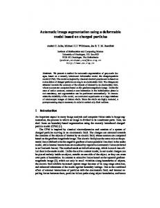
v. Computational Time: Time required for the Execution of the algorithm B. Block diagram of AISWT

Segmentation using ML Estimation

The Figure 1 gives the block diagram of AISWT I. Input image: The input images are of different formats, sizes and types. The image pixel intensity in the entire image is a Random Variable and follows a GGD. II. DWT: The Wavelet Transform is created by repeatedly filtering the image coefficients on a row by row and column by column basis. A two-dimensional DWT decomposition of image contains various band information such as low-low frequency approximation band, high-low frequency vertical detail band, low-high frequency horizontal detail band and high-high frequency diagonal detail band. We assume each coefficient of approximation band is a Random Variable z and also follow GGD. The approximation band is used for the segmentation purpose, which is quarter the size and has significant information of the original image. Hence the computation time required reduces. III. Initial parameters Estimation: Initial parameters like mean μ, variance σ and mixing parameter α are determined using Histogram based initial estimation which is a clustering algorithm. The initial parameters are calculated in two steps:

K Image Segments Fig 1: Block diagram of AISWT i) Histogram is constructed by dividing approximation band coefficients into intervals and counting the number of elements in each subspace, which is called as bin. The Khighest density bins are selected and the average of the observed elements belonging to the bins is calculated to derive a Centroid. If K centroids are not obtained because of narrow intervals, the Histogram is rebuilt using wider intervals and the centroids are recalculated. ii) The minimum distance clustering is used to label all the observed elements by calculating the distance D between each centroid and all the elements of the histogram as given in Equation (5) Dj = min||Ci – Yj|| ------------------------------- (5) Where Ci is ith centroid for i = 1 to K Dj is minimum distance between Ci and jth element Yj for j = 1 to N

IJCSNS International Journal of Computer Science and Network Security, VOL.9 No.2, February 2009 The Histogram based initial estimation do not use random selection for initial parameters, thus the method is stable and useful for unsupervised image segmentation applications. The obtained mean, variance and mixing parameter for the k regions are considered as the initial parameters for EM algorithm. IV. Shaping parameter P: The Shaping parameter defines the peakness of the distribution. In GGD, the three parameters mean, variance and shaping parameter determines the PDF. The optimal shaping parameter [22, 23] is determined using initial parameters and the absolute mean value E [ z ] . The absolute mean is given by

(

)

N

[ ( (

K

Q θ ,θ (i ) = ∑∑ log αt f zs ,θt(i ) tt zs ,θ (i )

N

Where

(

i =1 j =1

i

− μ j ------------------ (6)

P is estimated using Equation (7)

P = M −1 (ρ ) ---------------------------------- (7)

Where ρ is given by

ρ=

by Equation (10)

(

α t (i ) f z s , θ t (i ) tt (z s ,θ ) = h(z s ,θ (i ) ) (i )

K

∑α

h ( z s , θ (i ) ) =

t =1

------------- (10)

f ( z s , θ t(i ) )

(

Likelihood function Q θ , θ

α t (i+1) =

--- (11)

i

t

s =1

2

μt

(i + 1 )

=

s =1 N

i

t

s

s =1

t

s

Parameter

θ (0)

E-step

Q θ , θ (i )

(

)

M-step

)

(

Q θ ,θ (i +1)

θ = (α , μ ,σ 2 , P ).

(

Q θ ,θ

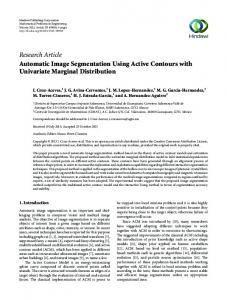
Each iteration of the EM algorithm consists of two steps as shown in Figure2

(i+1)

Is

) ~ Q(θ,θ ( ) ) < 0.001 i

Converged? Yes

i. E-step: It computes the expected complete data Log-

(

-------------- (13)

(i )

Choose an Initial

V. Expectation and Maximization: The EM algorithm is an efficient iterative procedure to compute the ML estimate in the presence of missing or hidden data. For obtaining the EM algorithm a sample of the coefficients z1, z,..., zn, are drawn with PDF f (z,θ) given in Equation (15) where θ is set of initial parameters

Likelihood function Q θ , θ

s

∑ t (z , θ )

⎛2⎞ Γ 2 ⎜⎜ ⎟⎟ ⎝ρ⎠ -------------------- (8) M (ρ ) = ⎛1⎞ ⎛3⎞ Γ ⎜⎜ ⎟⎟ Γ ⎜⎜ ⎟⎟ ⎝ρ⎠ ⎝ρ⎠

(i )

---------------- (12)

s

∑ t (z , θ ( ) ) z

)

(i )

∑ t (z ,θ ( ) ) N

1 N N

M is the Generalized Gaussian ratio function given by Equation (8)

i.e.,

t

)

ii. M-step: It finds the (i+1)th estimation θ by updating mixing parameter, mean and variance using Equations (12), (13) and (14) respectively to maximize Log-

E2[z ]

σ

------------ (9)

)

tt zs ,θ ( i ) is a Posterior Probability and is given

( i +1)

k

∑∑ z

)

s=1 t =1

Equation (6)

1 E[ z ] = N

))] (

309

) given by Equation (9)

Fig 2: Flow chart of EM .

No


310

1

σt

(i +1)

1 p ⎡ N (i ) P ⎤ (i ) ⎛ Γ(3 P ) ⎞ ⎜ ⎟ t z − , θ z μ ⎢∑ t s ⎥ t ⎜ PΓ(1 P ) ⎟ s s =1 ⎝ ⎠ ⎥ =⎢ N ⎢ ⎥ (i ) tt z s , θ ∑ ⎢ ⎥ s =1 ⎢⎣ ⎥⎦ ----- (14)

(

)

(

)

The EM algorithm will converge when the difference of the old estimates and the new estimates is less than the threshold value 0.001. The EM algorithm used for estimating the final parameters is heavily dependent on number of segments and the initial parameters of the model. VI. Generalized Gaussian Distribution model: The GGD model is obtained using the final parameters. The approximation band coefficients of each image region follow a particular distribution such as Gaussian, Laplacian, Uniform etc., and characterize the GGD Model with shaping parameter P. The PDF is given by Equation (15) ( zs −μi )

P

− 1 e A( P,σ ) --- (15) f (z,θ ) = ⎛ 1⎞ 2Γ⎜1 + ⎟ A(P,σ ) ⎝ P⎠

Where, s=1 to N and i=1 to K 1

⎡ 2 ⎛ 1 ⎞⎤2 ⎢ σ Γ⎜ P ⎟ ⎥ ⎝ ⎠⎥ for σ > 0, A(P, σ ) = ⎢ ⎛ ⎢ Γ⎜ 3 ⎞⎟ ⎥ ⎢⎣ ⎝ P ⎠ ⎥⎦ The function A(P, σ ) is a scaling factor and P is the shape parameter. The GGD becomes Laplacian Distribution if P = 1, Gaussian Distribution if P = 2 and Uniform Distribution if P→ +∞. VII. Segmentation using Maximum Likelihood Estimation: The segmentation is carried out by assigning each coefficient into proper cluster according to the ML estimation given by Equation (16)

L = maxt { f ( zs ,θ t )} -------------------- (16) VIII. K image segments: The K segmented regions are obtained and for K=2, the image is segmented into

foreground and background. The pixel intensities of segmented region obtained follow a corresponding GGD.

4. Algorithm Problem definition: Consider an image, the objectives are to i. Segment the given image using DWT. ii. Initial parameters are obtained using Histogram and EM iii. Segmentation is done using ML Estimation Assumption: Each coefficient of approximation band is a Random Variable z and also follows GGD Table 1 gives the AISWT Segmentation algorithm in which approximation band of image DWT is used to estimate parameters which are required for segmentation. Table 1 AISWT Algorithm • •

Input : Image of variable size Output : Segmented regions

1 DWT is applied on an image and approximation band is considered. 2 Histogram Based method is applied to obtain initial parameters like mean, variance and mixing parameter 3 Shaping parameter P is determined 4 Expectation and Maximization algorithm is used to get updated final parameters. 5 PDF of Generalized Distribution is determined

Gaussian

6 Segmentation is obtained using Maximum-Likelihood estimation.

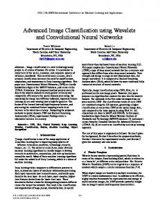
5. Performance Analysis Images Sea, Flower, Starfish and Boat of sizes 150*94, 127*127, 800*600 and 800*603 respectively are considered for performance analysis. If the number of segments are selected as two i.e., K=2 foreground and background can be differentiated in an image. Figures 3, 4, 5 and 6 gives the segmentation results of Sea, Flower, Starfish and Boat in which the original image, mask,


311

segment 1 and segment 2 are shown in Figures a, b, c and d respectively. Table 2 gives the comparison of computational time between FGM, FGGD and AISWT. It is observed that as dimension of the image increases, the computational time increases. The existing algorithms FGM and FGGD require more time compared to the proposed algorithm AISWT. AISWT requires 30% less time compared to FGM and 70% less time compared to FGGD.

a

b

c

d

Table 2: Comparison of Computational time for FGM, FGGD and AISWT Images Sea Flower Starfish Boat

FGM (sec) 1.53 1.57 39.9 38.84

FGGD (sec) 2.97 2.8 96.43 100.12

AISWT (sec) 0.9 0.9 26.5 27.2

Fig 4 a) original Flower (127*127) c) Segment 1 d) Segment 2

b) mask

Table 3 gives the comparison of Image quality Index between FGM, FGGD and AISWT. It is observed that proposed model AISWT has higher Image Quality Index compared to existing algorithms FGM and FGGD. a

b

c

d

a

b

Fig 3 a) Original Sea (150*94) b) Mask c) Segment 1 d) Segment 2 Table 3: Comparison of Image Quality Index for FGGD and AISWT Images Sea Flower Starfish Boat

FGM 93.7 95.5 88 90.9

FGGD 93.8 96 93.1 83

AISWT 97.3 98.6 95 91.3

FGM, c d Fig 5 a) original Starfish (800*600) b) Mask c) Segment 1 d) Segment 2


312

[6] [7]

a

b [8]

[9]

c d Fig 6 a) Original Boat (800*603) b) Mask c) Segment 1 d) Segment 2

6. Conclusion In this paper, we proposed fast segmentation algorithm AISWT. The approximation band of an image DWT is considered as a mixture of K-Component GGD. The initial parameters are estimated using Histogram based method. Through EM algorithm, the final parameters are obtained. The segmentation is done by ML estimation. The AISWT algorithm is computationally efficient for segmentation of large images and performs much superior to the earlier image segmentation methods FGM and FGGD in terms of computation time and image quality index.

[10]

[11]

[12]

[13]

[14]

Reference [1] E. Sharon, A. Brandt and R. Basri, “Fast Multi-Scale Image Segmentation,” Proceedings of the IEEE Conference on Computer Vision and Pattern Recognition, vol. 1, pp. 70-77, 2000 [2] P. V. G. D. Prasad Reddy, K. Srinivas Rao and S. Yarramalle, “Unsupervised Image Segmentation Method based on Finite Generalized Gaussian Distribution with EM and K-Means Algorithm,” Proceedings of International Journal of Computer Science and Network Security, vol.7, no. 4, pp. 317-321, April 2007. [3] L. O. Donnell, C. F. Westin, W. E. L. Grimson, J. R. Alzola, M. E. Shenton and R. Kikinis, “Phase-Based user Steered Image Segmentation,” Proceedings of the Fourth International Conference on Medical Image Computing and Computer-Assisted Intervention, pp. 1022-1030, 2001 [4] J. Bruce, T. Balch and M. Veloso, “Fast and Inexpensive Color Image Segmentation for Interactive Robots,” Proceedings of the IEEE International Conference on Intelligent Robots and Systems, vol. 3, pp. 2061-2066, 2000. [5] Z. Shi and V. Govindaraju, “Historical Handwritten Document Image Segmentation using Background Light

[15]

[16]

[17]

[18]

[19]

Intensity Normalization,” SPIE Proceedings on Center of Excellence for Document Analysis and Recognition, Document Recognition and Retrieval, vol. 5676, pp. 167174, January 2005. B. Sumengen and B. S. Manjunath, “Multi-Scale Edge Detection and Image Segmentation,” Proceedings of European Signal Processing Conference, September 2005. J. Malik, S. Belongie, J. Shi and T. Leung, “Textons, Contours and Regions: Cue Integration in Image Segmentation,” Proceedings of Seventh International Conference on Computer Vision, pp. 918-925, September 1999. P. F. Felzenswalb and D. P. Huttenlocher, “Efficient GraphBased Image Segmentation,” Proceedings of International Journal of Computer Vision, vol. 59, no. 2, pp. 167-181, 2004. J. Shi and J. Malik, “Normalized Cuts and Image Segmentation,” IEEE Transactions on Pattern Analysis and Machine Intelligence, vol. 22, no. 8, pp. 888-905, 2000. Y. Wu, X. Yang and K. L. Chan, “Unsupervised Color Image Segmentation based on Gaussian Mixture Models,” Proceedings of Fourth International Joint Conference on Information, Communications and Signal Processing, vol.1, no. 15, pp. 541-544, December 2003. T. Yamazaki, “Introduction of EM Algorithm into Color Image Segmentation,” Proceedings of International Conference on Intelligent Processing Systems, pp. 368-371, 1998. J. B. Mena and J. A. Malpica, “Color Image Segmentation using the Dempster-Shafer Theory of Evidence for the Fusion of Texture,” International Archives of Photogrammetry Remote Sensing and Spatial Information Sciences, vol. 34, pp. 139-144, 2003. B. Sumengen and B. S. Manjunath, “Graph Partitioning Active Contours for Image Segmentation,” IEEE Transactions on Pattern Analysis and Machine Intelligence, vol.28, no. 4, pp. 509-521, April 2006. M. Bakos, “Active Contours and their Utilization at Image Segmentation,” Proceedings of Fifth Slovakian-Hungarian Joint Symposium on Applied Machine Intelligence and Informatics, pp. 313-317, January 2007. T. Geraud, P. Y. Strub and J. Darbon, “Color Image Segmentation based on Automatic Morphological Clustering,” Proceedings of IEEE International Conference on Image Processing, vol. 3, pp. 70-73, October 2001. S. Wesolkowski, S. Tominaga and R. D. Dony, “Shading and Highlight Invariant Color Image Segmentation,” SPIE Color Imaging: Device-Independent Color, Color Hardcopy and Graphic Arts VI, pp. 229-240, January 2001. W. Cai, J. Wu and A. C. S. Chung, “Shape-Based Image Segmentation using Normalized Cuts,” proceedings of Thirteenth International Conference on Image Processing, pp. 1101-1104, October 2006. L. Bar, N. Sochen, and N. Kiryati, “Variational Pairing of Image Segmentation and Blind Restoration,” Proceedings of the European Conference on Computer Vision, vol. 3022, pp. 166-177, 2004. A. Mavrinac, “Competitive Learning Techniques for Color Image Segmentation,” Proceedings of the Machine Learning and Computer Vision, vol. 88, no. 590, pp. 33-37, April 2007.


313

[20] T. Cour, F. Benezit and J. Shi, “Spectral Segmentation with Multi-Scale Graph Decomposition,” IEEE Computer Society Conference on Computer Vision and Pattern Recognition, vol. 2, pp. 1124-1131, February 2005. [21] M. Ozden and E. Polat, “Image Segmentation using Color and Texture Features,” Proceedings of Thirteenth European Signal Processing Conference, September 2005. [22] J. A. D. Molina and R. M. R. Dagnino, “A Practical Procedure to Estimate the Shape Parameters in the Generalized Gaussian Distribution,” IEEE Transactions on Image Processing, pp. 1-18, 2003. [23] K. Sharifi and A. L. Garcia, “Estimation of Shape Parameter for Generalized Gaussian Distribution in Subband Decomposition of video,” IEEE Transactions on Circuits and Systems for Video Technology, vol. 5, no.1, pp. 52-56, 1995.

Bangalore University and Ph.D. in Computer Science from Indian Institute of Technology, Madras. He has a distinguished academic career and has degrees in Electronics, Economics, Law, Business Finance, Public Relations, Communications, Industrial Relations, Computer Science and Journalism. He has authored 27 books on Computer Science and Economics, which include Petrodollar and the World Economy, C Aptitude, Mastering C, Microprocessor Programming, Mastering C++ etc. He has been serving as the Professor and Chairman, Department of Computer Science and Engineering, University Visvesvaraya College of Engineering, Bangalore University, Bangalore. During his three decades of service at UVCE he has over 200 research papers to his credit. His research interests include computer networks, parallel and distributed systems, digital signal processing and data mining.

Bibliography

L M Patnaik is a Vice Chancellor, Defence Institute of Advanced Technology (Deemed University), Pune, India. During the past 35 years of his service at the Indian Institute of Science, Bangalore. He has over 500 research publications in refereed International Journals and Conference Proceedings. He is a Fellow of all the four leading Science and Engineering Academies in India; Fellow of the IEEE and the Academy of Science for the Developing World. He has received twenty national and international awards; notable among them is the IEEE Technical Achievement Award for his significant contributions to high performance computing and soft computing. His areas of research interest have been parallel and distributed computing, mobile computing, CAD for VLSI circuits, soft computing, and computational neuroscience.

Mr. H.C. SATEESH KUMAR is a Assistant Professor in the Dept of Telecommunication Engg, Dayananda sagar college of Engg, Bangalore. He obtained his B.E. degree in Electronics Engg from Bangalore University. His specialization in Master degree was “Bio-Medical instrumentation from Mysore University and currently he is pursuing Ph.D. in the area of Image segmentation under the guidance of Dr.K.B.Raja, Assistant Professor, Dept of Electronics and Communication Engg, University Visvesvaraya college of Engg, Bangalore. His area of interest is in the field of Signal Processing and Communication Engg. He is the life member of Institution of Engineers (India), Institution of Electronics and Telecommunication Engineers and Indian society for Technical Education. K B Raja is an Assistant Professor, Dept. of Electronics and Communication Engg, University Visvesvaraya college of Engg, Bangalore University, Bangalore. He obtained his Bachelor of Engineering and Master of Engineering in Electronics and Communication Engineering from University Visvesvaraya College of Engineering, Bangalore. He was awarded Ph.D. in Computer Science and Engineering from Bangalore University. He has over 35 research publications in refereed International Journals and Conference Proceedings. His research interests include Image Processing, Biometrics, VLSI Signal Processing, computer networks. K R Venugopal is currently the Principal and Dean, Faculty of Engineering, University Visvesvaraya College of Engineering, Bangalore University, Bangalore. He obtained his Bachelor of Engineering from University Visvesvaraya College of Engineering. He received his Masters degree in Computer Science and Automation from Indian Institute of Science Bangalore. He was awarded Ph.D. in Economics from