Shared Buffer Implementations of Signal Processing ... - CiteSeerX

October 4, 2000

To appear in the IEEE Transactions on Computer-Aided Design of Integrated Circuits and Systems.

Shared Buffer Implementations of Signal Processing Systems Using Lifetime Analysis Techniques Praveen K. Murthy Angeles Design Systems [email protected] Shuvra S. Bhattacharyya University of Maryland, College Park [email protected]

Abstract1 There has been a proliferation of block-diagram environments for specifying and prototyping DSP systems. These include tools from academia, such as Ptolemy, and commercial tools, such as DSPCanvas from Angeles Design Systems, SPW from Cadence, and COSSAP from Synopsys. The block diagram languages used in these environments are usually based on dataflow semantics because various subsets of dataflow have proven to be good matches for expressing and modeling signal processing systems. In particular, synchronous dataflow (SDF) has been found to be a particularly good match for expressing multirate signal processing systems. One of the key problems that arises during synthesis from an SDF specification is scheduling. Past work on scheduling from SDF has focused on optimization of program memory and buffer memory under a model that did not exploit sharing opportunities. In this paper, we build on our previously developed analysis and optimization framework for looped schedules to formally tackle the problem of generating optimally compact schedules for SDF graphs. We develop techniques for computing these optimally compact schedules in a manner that also attempt to minimize buffering memory under the assumption that buffers will be shared. This results in schedules whose data memory usage is drastically lower than methods in the past have achieved. The method we use is that of lifetime analysis; we develop a model for buffer lifetimes in SDF graphs, and develop scheduling algorithms that attempt to generate schedules that minimize the maximum number of live tokens under the particular buffer lifetime model. We develop several efficient algorithms for extracting the relevant lifetimes from the SDF schedule. We then use the well-known firstfit heuristic for packing arrays efficiently into memory. We report extensive experimental results on applying these techniques to several practical SDF systems, and show improvements that average 50% over previous techniques, with some systems exhibiting up to an 83% improvement over previous techniques.

1

Introduction Block diagram environments are proving to be increasingly popular for developing DSP systems.

The reasons for their popularity are many: block-diagram languages are visual and hence intuitive to use for engineers naturally used to conceptualizing systems as block diagrams, block diagram languages promote software reuse by encapsulating designs as modular, reusable components, and finally, these lan1. A portion of Shuvra Bhattacharyya’s research was sponsored by the US National Science Foundation (9734275)

1 of 42

Introduction

guages can be based on models of computation that have strong formal properties, enabling easier and faster development of bug-free programs. Block-diagram specifications also have the desirable property of not over-specifying systems; this can enable a synthesis tool to exploit all of the concurrency and parallelism available at the system level. In a block-diagram environment, the user connects up various blocks drawn from a library to form the system of interest. For simulation, these blocks are typically written in a high level language (HLL) like C++. For software synthesis, the technique typically used is that of inline code generation: a schedule is generated, and the code generator steps through this schedule and substitutes the code for each actor that it encounters in the schedule. The code for the actor may be of two types. It may be the HLL code itself, obtained from the actor in the simulation library. The overall code may now be compiled for the appropriate target. Or the code may be hand-optimized code targeted for a particular target implementation. For programmable DSPs, this means that the actors implement their functionality through hand-optimized assembly language segments. The code-generator, after stitching together the code for the entire system then simply assembles it and the resulting machine code can be run on the DSP. This latter technique is generally more efficient for programmable DSPs because of a lack of efficient HLL DSP compilers. For hardware synthesis, a similar approach can be taken, with blocks implementing their functionality in a hardware description language, like behavioral VHDL [12][34]. The generated VHDL description can then be used by a behavioral synthesis tools to generate an RTL description of the system, that can be further compiled into hardware using logic synthesis and layout tools. High-level language compilers for DSPs have been woefully inadequate in the past [35]. This has been because of the highly irregular architecture that many DSPs have, the specialized addressing modes such as modulo addressing, bit-reversed addressing, and small number of special purpose registers. Traditional compilers are unable to generate efficient code for such processors. This situation might change in the future, if DSP architectures converge to general-purpose architectures; for example, the C6 DSP from TI, the newest DSP architecture from TI, is a VLIW architecture and has a fairly good compiler. Even so, because of low power requirements, and cost constraints, the fixed-point DSP with the irregular architecture is likely to dominate in embedded applications for the foreseeable future. Because of the shortcomings of existing compilers for such DSPs, a considerable research effort has been undertaken to design better compilers for fixed point DSPs (e.g., see [19][20][21]). Synthesis from block diagrams is useful and necessary when the block diagram becomes the abstract specification rather than C code. Block diagrams also enable coarse-grain optimizations based on knowledge of the restricted underlying models of computation; these optimizations are frequently difficult 2 of 42

Shared Buffer Implementations of Signal Processing Systems Using Lifetime Analysis Techniques

Problem statement and organization of the paper

to perform for a traditional compiler. Since the first step in block diagram synthesis flows is the scheduling of the block diagram, we consider in this paper scheduling strategies for minimizing memory usage. Since the scheduling techniques we develop operate on the coarse-grain, system level description, these techniques are somewhat orthogonal to the optimizations that might be employed by tools lower in the flow. For example, a behavioral synthesis tool has a limited view of the code, often confined to basic blocks within each block it is optimizing, and cannot make use of the global control and dataflow that our scheduler can exploit. Similarly, a compiler for a general-purpose HLL (such as C) typically does not have the global information about application structure that our scheduler has. The techniques we develop in this paper are thus complementary to the work that is being done on developing better HLL compilers for DSPs, such as that presented in [19][20][21]. In particular, the techniques we develop operate on the graphs at a high enough level that particular architectural features of the target processor are largely irrelevant. We assume that the actor library that the code generator has access to consists of either hand-optimized assembly code, or of specifications in a high-level language like C. If the latter, then we would have to invoke a C compiler after performing the dataflow optimizations and threading the code together. Even though this might seemingly defeat the purpose of producing efficient code, since we are using a C compiler for a DSP (the compiler might not be very good as mentioned), studies have shown that for larger systems, C code produced this way compiles better than hand-written C for the entire system [15].

2

Problem statement and organization of the paper In this paper, we describe a technique for reducing buffering requirements in synchronous data-

flow (SDF) graphs based on lifetime analysis and memory allocation heuristics for single appearance looped schedules (SAS). As already mentioned, the first step in compiling SDF graphs is determining a schedule. Once the schedule has been determined, memory has to be allocated for the buffers in the graph. Both of these steps present many algorithmic challenges; we tackle many of these steps in this paper. We concentrate on the class of single appearance schedules in our framework because non-single appearance schedules for SDF graphs can be exponentially long; this can lead to very large code size [4]. Within the class of SAS, there are two algorithmic challenges: to determine the order in which the actors should appear in the schedule, subject to the precedence constraints imposed by the graph (the topological ordering), and the order in which the loops should be organized once the order has been determined. Solutions to both of these problems depend on the optimization metric of interest. In this paper, the metric is buffer memory; hence, these algorithms all try to minimize the amount of buffer memory needed. While previous techniques for buffer minimization have used techniques where each buffer is allocated independently in memory (we will refer to this as the non-shared model), in this paper we try to share buffers efficiently by Shared Buffer Implementations of Signal Processing Systems Using Lifetime Analysis Techniques

3 of 42

Problem statement and organization of the paper

using lifetime analysis techniques (referred to as the shared model). In the memory allocation steps, the challenges are to efficiently extract buffer lifetimes from the schedule, and to pack these buffers into memory efficiently. All of the algorithms we present are provably polynomial-time algorithms; this is important because SDF compilers are often used in rapid-prototyping environments where fast compile times are necessary and desirable. In section 3 we review relevant past work on this subject. Sections 4 and 5 establish some of the notation and definitions we will use. Figure 1 summarizes the various algorithms that we will develop in this paper as part of our SDF compiler framework. The box with “RPMC and APGAN” in figure 1 finds the topological ordering and is reviewed in section 7 (briefly since these algorithms have been developed previously). The box with “SDPPO” solves the loop ordering problem and is described in section 7. After the SDPPO step, we will have a theoretical idea of the amount of buffer memory required, but as will be shown, until the actual memory allocation is performed, we do not know the exact requirements. The memory allocation steps take the schedule produced by the first two steps and attempt to determine the most efficient allocation. In order to do this, we have to build a tree representation of the schedule; this is covered in section 5. On this representation, several parameters that are needed for lifetime analysis, like the start and stop times of buffers, their periodicities, and durations have to be computed; algorithms for doing this efficiently are given in section 8. Once all of the lifetime parameters have been determined, another structure called an intersection graph has to be built. On this graph, allocation heuristics are applied in order to get a final memory allocation; these two steps are covered in section 9. Since we have developed two efficient heuristics for generating topological orderings in the scheduling step, neither of which can be said to be clearly superior, and since we have developed two heuristics that can be used in the memory allocation step, our experiments in section 10 examine all four of the possible combinations to

SDF Graph

Determine topological ordering (RPMC or APGAN)

Loop Fusion for memory reduction (SDPPO)

Scheduling steps

Code generation

Build schedule tree

Compute buffer widths, durations, start, stop times, periods, and period bounds

Memory allocation steps Storage allocation (first fit)

Build intersection graph

Fig 1. Flow chart showing the sequence in which the various algorithms are applied. 4 of 42


Related Work

determine the most efficient combination for each test example. In section 11 we discuss possibilities for future work and conclude.

3

Related Work Lifetime analysis techniques for sharing memory are well known in a number of contexts. The first

is for register allocation in traditional compilers; given a scheduled dataflow graph, register allocation techniques determine whether the variables in the graph can be shared by looking at their lifetimes. In the simplest form, this problem can be formulated as an interval graph coloring problem that has an elegant polynomial-time solution. However, the problem of scheduling the graph so that the overall register requirement is minimized is an NP-hard problem [30]. Register allocation problems are made somewhat simpler because the variables in question all have the same size. The allocation problem becomes NP-complete if variables are of differing sizes, as for example, in allocating arrays of different sizes to memory. Fabri[8] studies the more general problem of overlaying arrays and strings in imperative languages. Fabri models array lifetimes as weighted interval graphs and uses coloring heuristics for generating memory allocations. She also studies transformation techniques for lowering the overall memory cost; these techniques attempt to minimize the lower and upper bounds on the extended chromatic number of the weighted interval graph. Some transformation techniques found to be effective for reducing overall storage include the renaming transformation, where by the use of judicious renaming of aggregate variables, lifetimes can be fragmented, allowing greater opportunities for overlaying; the technique of recalculation, where some variables are recalculated when needed, rather than holding them in storage; code motion techniques that reorder the program statements in a semantics preserving manner; and loop splitting. There are important differences between Fabri’s work and ours. Fabri considers general imperative language code, and hence has to solve allocation problems for a more general class of interval graphs. We apply our techniques on SDF graphs, and because the SDF model of computation is restricted, the interval graphs in our problem have a more restricted structure, enabling us to use simpler allocation heuristics more effectively. For instance, the liveness profile of an array in our framework is always periodic (in a certain technical sense), and these periods can be deduced from the SDF graph and the specific class of schedules that we use, whereas in a general setting, liveness profiles may not be periodic, and deducing these profiles can be expensive algorithmically. Also, the SDF model and SDF schedules present unique problems for deducing the liveness profiles, and thus the interval graphs, in an efficient manner; these techniques have not been presented or studied in any previous work. We show that for the important class of single appearance schedules, these deductions can be made in polynomial time in the size of the SDF Shared Buffer Implementations of Signal Processing Systems Using Lifetime Analysis Techniques

5 of 42

Related Work

graph. We present an optimization technique for reducing the extended chromatic number by performing loop fusion in a systematic manner. While the loop fusion technique is applicable in a general setting as well, opportunities for doing it in a general setting do not arise as frequently and naturally as they do in an SDF setting; hence, it is a very effective technique here. For example, determining the applicability of loop fusion is undecidable in procedural languages; whereas exact analysis is decidable and tractable in our context. Thus loop fusion is more effective for SDF graphs, and our work exploits this increased effectiveness. Also, previous work has not addressed the relationship been loop fusion and the extended chromatic number. Finally, even though certain subsets of the techniques we present in this paper have been studied in the compilers community, to date they have not been used in block-diagram compilers. An additional contribution of this paper is to show that many of the techniques used in traditional compilers can be specialized and applied fruitfully in block diagram based DSP programming environments. Vanhoof, Bolsens and De Man have observed that in general, the full address space of an array does not always contain live data [33]. Thus, they define an "address reference window" as the maximum distance between any two live data elements throughout the lifetime of an array, and fold multiple array elements into a single window element using a modulo operation in the address calculation. This concept is similar to our use of the maximum number of live tokens as the size of each individual SDF buffer. The number of logically distinct memory elements in a buffer for an edge e is equal to TNSE ( e ) , which can be much larger than the maximum number of live tokens that reside on e simultaneously [4]. In a synthesis tool called ATOMIUM, De Greef, Catthoor, and De Man have developed lifetime analysis and memory allocation techniques for single-assignment, static control-flow specifications that involve explicit looping constructs, such as for loops [11]. This is in contrast to SDF, in which all iteration is specified implicitly, and the use of looping is left entirely up to the compiler. However, once a single appearance schedule is specified, we have a set of nested loops. Thus, some relationships can be observed between the lifetime analysis techniques we develop for single appearance schedules, and those of ATOMIMUM. In particular, the class of specifications addressed by ATOMIUM exhibits more general and less predictable array accessing behavior than the buffer access patterns that emerge from SDF-based single appearance schedules. We exploit the increased predictability of single appearance schedules in our work using novel lifetime analysis formulations that are derived from a tree-based schedule representation. This results in thorough optimization with significantly more efficient (lower complexity) algorithms. Furthermore, through our in-depth focus on the restricted, but useful, class of SDF-based single appearance schedules, we expose fundamental relationships between scheduling and buffer sharing in multirate signal processing systems.

6 of 42


Related Work

Ritz et al. [29] give an approach to minimizing buffer memory that operates only on flat SASs since buffer memory reduction is tertiary to their goal of reducing code size and context-switch overhead (defined roughly as the rate at which the schedule switches between various actors). We do not take context-switch into account in our scheduling techniques because our primary concern is memory minimization; off-chip memory is often a bottleneck in embedded systems implementations and is better avoided. Flat SASs have a smaller context switch overhead then nested schedules do, especially if the codegeneration strategy used is that of procedure calls. Ritz et al. formulate the problem of minimizing buffer memory on flat SASs as a non-linear integer programming problem that chooses the appropriate topological sort and proceeds to allocate based on that schedule. This formulation does not lead to any polynomialtime algorithms, and can lead to much more expensive memory allocations than those obtainable through nested schedules. For example, in Section 10, we show that on a satellite receiver example, Ritz’s technique yields an allocation that is more than 100% larger than the allocation achieved by techniques developed in this paper. However, the techniques in this paper do not take context-switch overhead into account (since we assume inline code generation, the effect of context switches is arguably less significant), and are thus able to operate on a much larger class of SASs than the class of flat SASs. Also, the techniques in this paper are all provably polynomial-time algorithms. Goddard and Jeffay use a dynamic scheduling strategy for reducing memory requirements of SDF graphs, and develop an earliest-deadline-first (EDF) type of dynamic scheduler [10]. However, experiments in the Ptolemy system have shown that dynamic scheduling can be more than twice as slow as static schedules [36]; hence, for many embedded applications, this penalty on throughput might be intolerable. Sung et al. consider expanding the SAS to allow 2 or more appearances of some actors if the buffering memory can be reduced [31]. They give heuristic techniques for performing this expansion and show that the buffering can be reduced significantly by allowing an actor to appear more than once. This technique is useful since it allows one to trade-off buffering memory versus code size in a systematic way. SASs will give the least code size only if each actor in the schedule is distinct and has a distinct codeblock that implements its functionality. In reality, however, many actors in the graph will be different instantiations of the same basic actor, with different parameters perhaps. In this case, inline code generated from a SAS is not necessarily code-size optimal since the different instantiations of a single actor could all share the same code [31]. Hence, it might be profitable to implement procedure calls instead of inline code for the various instantiations, so that code can be shared. The procedure call would pass the appropriate parameters. A study of this optimization is done in [31] where the authors formulate precise metrics that can be used to determine the gain or loss from implementing code sharing compared to the overhead of Shared Buffer Implementations of Signal Processing Systems Using Lifetime Analysis Techniques

7 of 42

Notation and background

using procedure calls. Clearly, all of the scheduling techniques mentioned in this paper can use this codesharing technique also, and our work is complementary to this optimization. Ade has developed lower bounds on memory requirements of SDF specifications, assuming that each buffer is assigned to separate storage [1]. Exploring the incorporation of buffer sharing opportunities into this analysis is a useful direction for further investigation. As already mentioned, dataflow is a natural model of computation to use as the underlying model for a block-diagram language for designing DSP systems. The blocks in the language correspond to actors in a dataflow graph, and the connections correspond to directed edges between the actors. These edges not only represent communication channels, conceptually implemented as FIFO queues, but also establish precedence constraints. An actor fires in a dataflow graph by removing tokens from its input edges and producing tokens on its output edges. The stream of tokens produced this way corresponds naturally to a discrete time signal in a DSP system. In this paper, we consider a subset of dataflow called synchronous dataflow (SDF)[17]. In SDF, each actor produces and consumes a fixed number of tokens, and these numbers are known at compile time. In addition, each edge has a fixed initial number of tokens, called delays.

4

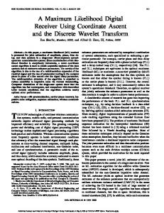
Notation and background Fig. 2(a) shows a simple SDF graph. Each edge is annotated with the number of tokens produced

(consumed) by its source (sink) actor, and the “10 D” on the edge from actor A to actor B specifies 10 delays. Each unit of delay is implemented as an initial token on the edge. Given an SDF edge e , we denote the source actor (that writes tokens on the edge), sink actor (that reads tokens from the edge), and delay of e by src ( e ) , snk ( e ) , and del ( e ) . Also, prod ( e ) and cns ( e ) denote the number of tokens produced onto e by src ( e ) and consumed from e by snk ( e ) . An SDF graph is called homogenous if prod ( e ) = cns ( e ) for all edges e . A schedule is a sequence of actor firings. We compile an SDF graph by first constructing a valid schedule — a finite schedule that fires each actor at least once, does not deadlock, and produces no net change in the number of tokens queued on each edge. Corresponding to each actor in the schedule, we instantiate a code block or procedure call that is obtained from a library of predefined actors. The resulting Valid Schedules

A

10D 20

10 (a)

B

10

30

C

(1): BABBCABBABC

(2): 3(A 2B) 2C

(3): (3A) (6 B) (2 C)

(4): B A 2(A B) C 3B C (b)

Fig 2. (a) An example of an SDF graph. (b) Some valid schedules. 8 of 42


Constructing memory-efficient loop structures

sequence of code blocks is encapsulated within an infinite loop to generate a software implementation of the SDF graph. SDF graphs for which valid schedules exist are called consistent SDF graphs. In [4], efficient algorithms are presented to determine whether or not a given SDF graph is consistent, and to determine the minimum number of times that each actor must be fired in a valid schedule. We represent these minimum numbers of firings by a vector q G , indexed by the actors in G (we often suppress the subscript if G is understood). These minimum numbers of firings can be derived by finding the minimum positive integer solution to the balance equations for G , which specify that q must satisfy prod ( e )q [ src ( e ) ] = cns ( e )q [ snk ( e ) ] , for every edge e in G . The vector q , when it exists, is called the repetitions vector of G . A schedule is then a sequence of actor firings where is each actor v is fired q [ v ] times, and the firing sequence obeys the precedence constraints imposed by the SDF graph. For the graph is figure 2, we have q = [ 3, 6, 2 ] for the actors [ A, B, C ] , and some schedules are BABBCABBABC , AAABBBBBBCC , and BAAABBCBBBC . We define TNSE ( e ) to be the total number of samples exchanged on edge e by actor snk ( e ) ; i.e, TNSE ( e ) = q [ snk ( e ) ] ⋅ cns ( e ) .

5

Constructing memory-efficient loop structures In [4], the concept and motivation behind single appearance schedules (SAS) has been defined

and shown to yield an optimally compact inline implementation of an SDF graph with regard to code size (neglecting the code size overhead associated with the loop control). An SAS is one where each actor appears only once when loop notation is used. If the SAS restriction is removed, significant increase in code size can occur. The increase in code size will manifest itself even if inline code-generation is not used and subroutine calls are used instead. This is because the length of a non-SAS can be exponential in the size of the graph, and there could be exponentially many subroutine calls. Figure 2(b) shows some valid schedules for the graph in figure 2(a). The notation 2C represents the firing sequence CC . Similarly, 3 ( A ( 2B ) ) represents the schedule loop with firing sequence ABBABBABB . We say that the iteration count of this loop is 3 , and the body of this loop is A ( 2B ) . Schedules 2 and 3 in figure 2(b) are single appearance schedules since actors A, B, C appear only once. An SAS like the third one in figure 2(b) is called flat since it does not have any nested loops. In general, there can be exponentially many ways of nesting loops in a flat SAS [4].


9 of 42

Constructing memory-efficient loop structures

Scheduling can also have a significant impact on the amount of memory required to implement the buffers on the edges in an SDF graph. For example, in figure 2(b), the buffering requirements for the four schedules, assuming that one separate buffer is implemented for each edge, are 50, 90, 130, and 80 respectively. As can be seen, SASs can have significantly higher buffer requirements than a schedule optimized purely for buffer memory. For example, the non-SAS BABBCABBABC for the SDF graph of figure 2 has a buffer requirement of 50; the three possible SASs for the graph, 3A 6B 2C , 3 ( A 2B )2C , and 3A 2 ( 3B C ) , have requirements of 130, 90, and 100 respectively. We give priority to code-size minimization over buffer memory minimization; justification for this may be found in [4][24]. Hence, the problem we tackle is one of finding buffer-memory-optimal SASs, since this will give us the best schedule in terms of buffer-memory consumption amongst the schedules that have minimum code size.

5.1

R-Schedules and the Schedule Tree

In order to extract buffer lifetimes efficiently, we develop a useful representation of the nested SAS, called the schedule tree. The lifetime extraction algorithms of section 8 can then be formulated as tree-traversing algorithms for determining the various required parameters. As shown in [24], it is always possible to represent any SAS for an acyclic graph as (iLSL )(iRSR ) ,

(EQ 1)

where S L and S R are SASs for the subgraph consisting of the actors in S L and in S R , and i L and i R are iteration counts for iterating these schedules. In other words, the graph can be partitioned into a left subset and a right subset so that the schedule for the graph can be represented as in equation 1. SASs having this form (in conjunction with some additional technical restrictions on the loop iteration counts) at all levels of the loop hierarchy are called R-schedules [24]. Given an R-schedule, we can represent it naturally as a binary tree; we call this the schedule tree. The internal nodes of this tree will contain the iteration count of the subschedule rooted at that node. The leaf nodes (nodes that have no children) will contain the actors, along with their residual iteration counts. If a node v has children, we refer to the left child and right child of v by left ( v ) and right ( v ) . For a node u , the parent is referred to as parent ( u ) . Figure 3 shows schedule trees for the SASs in figure 2(b). Note that a schedule tree is not unique since if there are iteration counts of 1, then the split into left and 1

3(A 2B) 2C

2C

3 A

2B

1

3A 6B 2C 3A

1 6B

2C

Fig 3. Schedule trees for schedules (2) and (3) in figure 2(b). 10 of 42


Generating single appearance schedules

right subgraphs can be made at multiple places. In figure 3, the schedule tree for the flat SAS in figure 2(b)(3) is based on the split { A } { B, C } . However, we could also take the split to be { A, B } { C } . However, the split will not affect any of the computations we perform using the tree. If v is a node of the schedule tree, then subtree ( v ) is the (sub)tree rooted at node v . If T is a subtree, define root ( T ) to be the root node of T . The function loop:V → Z , where V is the set of nodes in the tree, and Z is the set of positive integers, returns for a non-leaf node, the iteration count at that nesting level, and returns 1 for a leaf node.

6

Generating single appearance schedules We have shown [4] that for an arbitrary acyclic graph, an SAS could be derived from a topological

sort of the graph. To be precise, the class of SASs for a delayless acyclic graph can be generated by enumerating the topological sorts of the graph. We use the lexical ordering given by each topological sort to derive a flat SAS (this is a schedule of the form ( q 1 x 1 ) ( q 2 x 2 )… ( q n x n ) , where the x i are actors and q i are the repetitions q [ x i ] . The lexical order x 1 x 2 …x n is the order given by the topological sort of the graph.). This lexical ordering then leads to a set of nesting hierarchies; the complete set of lexical orders and for each lexical order, the set of nesting hierarchies, constitutes the entire set of SASs for the graph. Hence, we need a method for generating the topological sort. As we have shown [4], the general problem of constructing buffer-optimal SASs under both models of buffering, namely the coarse shared buffer model, and the non-shared model, is NP-complete. Thus, the methods for generating topological sorts are necessarily heuristic, and not-optimal in general. We have developed two methods for generating SAS optimized for non-shared buffer memory for acyclic graphs [4]: a bottom-up method based on clustering called APGAN, and a top down method based on graph partitioning called RPMC. The heuristic rule-of-thumb used in RPMC is to find a cut of the graph such that all edges cross in the same direction (enabling us to recursively schedule each half without introducing deadlock), and such that size of the buffers crossing the cut is minimized. While this rule is intuitively attractive for the non-shared buffer model, it is also attractive for the shared model as will be shown. The APGAN technique is based on clustering adjacent nodes together that communicate heavily, so that these nodes will end up in the innermost loops of the loop hierarchy. For a broad subclass of SDF systems, APGAN has been shown to construct SAS that provably minimize the non-shared buffer memory metric over all SAS [4].


11 of 42

Efficient loop fusion for minimizing buffer memory

An arbitrary SDF graph may not necessarily have an SAS; Bhattacharyya et. al. developed necessary and sufficient conditions for the existence of SAS for SDF graphs [5]. They developed an algorithm for generating single appearance schedules that hierarchically decomposes the SDF graph into strongly connected components (SCC) and recursively schedules each SCC. At each stage, the SCC decomposition results in an acyclic component graph that has an SAS as mentioned, and can be scheduled using any algorithm for generating SAS for acyclic graphs. Hence, the techniques we develop in this paper can all be incorporated into the framework of [5] and can handle arbitrary SDF graphs.

7

Efficient loop fusion for minimizing buffer memory Once we have a topological order generated by APGAN or RPMC, we have a flat single appear-

ance schedule corresponding to this topological order. The next step is to perform loop fusion on the flat SAS to reduce buffering memory. To do that, we first define the shared buffer model.

7.1

The shared buffer model Since we are interested in sharing buffers, we have to first determine an appropriate model for

buffer lifetimes and the manner in which they can be shared. First, we need a definition for describing token traffic on the edges: given an SDF graph G , a valid schedule S , and an edge e in G , let max_tokens ( e, S ) denote the maximum number of tokens that are queued on eduring an execution of For

example,

if

for

fig.

2,

S 3 = ( 3A ) ( 6B ) ( 2C )

and

S 2 = 3 ( A 2B ) ( 2C ) ,

.S then

max_tokens ( ( A, B ), S 3 ) = 70 and max_tokens ( ( A, B ), S 2 ) = 30 . Buffer sharing for looped schedules can be done at many different levels of “granularity.” At the finest level of granularity, we can model the buffer on the edge as it grows over the execution of the loop, and then falls as the sink actor on that edge consumes the data. The maximum number of live tokens would give the lower bound on how much memory would be required. An alternative model would be at the coarsest level, where we assume that once the source actor for an edge e starts writing tokens, max_tokens ( e, S ) tokens immediately become live, and stay live until the number of tokens on the edge becomes zero, where S is the schedule. In other words, even if there is one live token on the edge, we assume that an array of size max_tokens ( e, S ) has to be allocated and maintained until there are no live tokens. Figure 4 shows these two extremes pictorially for the buffer on edge BC . In the fine-grained case, each firing of B results in the buffer on BC expanding by 5, and each firing of C results in the buffer contracting by 2. In the coarse-grained case, the buffer expands to 30 immediately as all 6 firings of B are treated as one composite firing, and then shrinks to 0 after all 15 firings of C have occurred. Of-course, there are a number of granularities within these extremes, based on how many levels of loop nests we con12 of 42



sider; figure 4 shows the in-between alternative for this example, where only the outer loop of iteration count 2 is considered, meaning that the three firings of B in the inner loop are treated as one composite firing. The buffer, in this case, expands by 3 × 5 = 15 tokens on each composite firing of B , and contracts by 5 × 2 = 10 on each composite firing of C consisting of 5 firings. In this paper, we assume the coarsest level of buffer modeling. The finer levels, although requiring less memory theoretically, may be practically infeasible to achieve due to the increased complexity of the algorithms. To see that the complexity might significantly increase, notice that the finest level requires modeling to be done at the granularity of single firing of an actor in the schedule. The number of firings in a periodic SDF schedule is O ( P m ) , where P = MAX e ∈ E { prod ( e ), cns ( e ) } , E is the set of edges in the SDF graph, and m = E . Of-course, there may be more clever ways of representing the growth and shrinkage, but presently the only known ways are equivalent to stepping through a schedule of size O ( P m ) . Clearly, this is an exponential function in the size of the SDF graph, and can grow quickly. In contrast, we will show that the coarsest level model can be generated in time polynomial in the number of nodes and edges in the SDF graph. One weakness of the coarse buffer sharing model is the assumption that all output buffers of an actor are live when the actor begins execution, and all input buffers are live until the actor finishes execution. This means that an output buffer of an actor can never share an input buffer of that actor under the model used in this paper. In reality, this may be an overly restrictive assumption; for instance, an addition actor that adds two quantities will always produce its output after it has consumed its inputs. Hence, the output result can occupy the space occupied by one of the inputs. We have formalized this idea, and have devised another technique called buffer merging [23] that merges input and output buffers by algebraically determining precisely how many output tokens are simultaneously live with input tokens (via a formalism called the consumed-before-produced (CBP) parameter [3]). The buffer merging technique is similar in spirit to the array merging technique presented by DeGreef et. al[11]; however it is more efficient in some ways, and also exploits distinguishing characteristics of SDF schedules in a novel way. We Actor firing according to schedule 3 A

5

5 B

2

3 C

Schedule: 2(5A 3B) 3(5C 3D)

5 D

A A B B B A A B B B C C

Tokens in buffer 5 15 20 30

5A 3B 5A 3B 5C 3D 5C 3D 5C 3D

15 30 20 10

5A 3B 5A 3B 5C 3D 5C 3D 5C 3D

30

28

Buffer BC Fine-grained model

An in-between model

Buffer BC Coarse-grained model

Fig 4. The fine-grained, in-between, and coarse-grained models of buffer sharing. Shared Buffer Implementations of Signal Processing Systems Using Lifetime Analysis Techniques

13 of 42


have shown that the buffer merging technique is highly complementary to the approach taken in this paper, and is in effect, a dual of the lifetime analysis approach because buffer merging works at the level of a single input/output edge pair, whereas the lifetime analysis approach of this paper works on a global level where the buffering efficiency results from the topology of the graph and the structure of the schedule [22, 23]. Initial tokens on edges can be handled very naturally in our coarse shared buffer model. An edge that has an initial token will have a buffer that is live right at the beginning of the schedule. It may be live for the entire duration of the schedule if the buffer never has zero tokens. If the buffer does have zero tokens at some point, then the buffer would be not be live for the portion of the schedule where the buffer has zero tokens. In order to reason about the “start time” and “stop time” of a buffer lifetime, we use the following abstract notion of time: each invocation of a leaf node in the schedule tree is considered to be one schedule step, and corresponds to one unit of time. For example, the looped schedule 2 ( A 3B ) would be considered to take 4 time steps. This is because the firing sequence is A 3B A 3B , and since the schedule loop 3B is a leaf node in the schedule tree, it is considered to take one schedule step. The first invocation of A would take place at time 0, and the last invocation of 3B begins at time 3 and ends at time 4. Note that this notion of time is not used to judge run-time performance of the schedule in terms of throughput; it is simply used to define the lifetimes for purposes of lifetime analysis. Figure 5 shows the anatomy of a buffer lifetime. Notice that this buffer becomes live several times. The start time is defined as the very first time the buffer becomes live; in this contrived example, at time 10. The stop time is defined as the very first time the buffer stops being live; at time 12 in the example. The duration is simply the difference between the stop and start times. The periodicity is modeled by a 3-tuple as shown; this will be described in greater detail in section 8.4. Briefly, it is modeled by a Diophantine Memory

“Time”

10 12 13 15 Width 20 22 23

Start time = 10 Duration = 2 Stop time = 12 Periodicity = [10, {3,10}, {2,2}] 0 p id but s ( p c ) < s ( p d ) . We have 0 < s ( p d ) – s ( p c ) = a 1b ( p 1d – p 1c ) + … + a ib– 1 ( p id– 1 – p ic– 1 ) + a ib ( p id – p ic ) ≤ a 1b p 1d + … + a ib– 1 p id– 1 – a ib < 0 by lemma 1 again, contradicting our assumption that p ic > p id . QED. 8.4.1

An algorithm for computing buffer liveness at a particular time

Given lemma 1, equation 5 can be solved by the algorithm in figure 15. The algorithm first subtracts the start time of the buffer since all computations can be made relative to the start time. It then simply determines the maximum p ib ∈ { 0, …, loop ( v ib ) – 1 } factor for each a ib , to determine the closest starting point of an occurrence of the periodic interval to time T . Claim 1: T' ≥ 0 at every stage in the algorithm. Proof: Note that p i ≤ T' ⁄ a ib for all i . Hence T' – p i a ib ≥ T' – T' ⁄ a ib a ib ≥ 0 . QED. Claim 2: The solution p i computed by the algorithm gives the starting point of the interval closest to T' . Proof: Let p be the tuple consisting of the p i . This means that any tuple p' > p gives an interval of starting time greater than T' . Indeed, suppose not and there is a tuple p' > p where s ( p ) < s ( p' ) < T' . Then, p' j > p j for the largest index j where the two tuples differ. Till the j th step, the value of T' computed by the algorithm would be identical to the computation using the values from p' . When i = j , the algorithm comGiven: a time T . Determine if a periodic buffer b parametrized by { start ( b ), ( a 1b, …, a nb ), ( loop ( v 1b ), …, loop ( v nb ) ) }

Buffer not live at T’

Buffer live at T’

is live at this time. Define T' ← T – start ( b ) . for i = n to 1 step -1  T'  p i ← min  ----, loop ( v ib ) – 1  a ib 

s( p ) T'

T' ← T' – p i a ib end for if ( T' < dur ( b ) ), then b is live ( p iare the solution) else not live.

s ( p ) + dur ( b )

Fig 15. An algorithm to determine whether a periodic buffer is live at a particular time. The depiction on the right shows two possibilities for the computed start time by the algorithm in relation to T' . Shared Buffer Implementations of Signal Processing Systems Using Lifetime Analysis Techniques

27 of 42

Creating the interval instances from a single appearance schedule

putes p j = min ( T' ⁄ a jb , loop ( v jb ) – 1 ) . Suppose p j = T' ⁄ a jb . Clearly, anything larger than p j will mean that T' – p j a jb < 0 , giving a start time greater than T' . If p j = loop ( v jb ) – 1 , then we cannot have p' j > p j since loop ( v jb ) – 1 is the largest value the j th component is allowed to take by definition. Hence, we cannot have p' j > p j , contradicting the assumption that p' > p . QED. The last step of the algorithm checks whether T' < dur ( b ) to determine whether the interval with closest starting time less than or equal to T' is still alive. If b is not live at time T , we will need to determine when the next instance of its periodic interval will occur. This computation is needed to determine whether some other interval of a particular duration is completely disjoint with the set of intervals corresponding to b — that is, to determine whether some other interval can be fitted into the same location that b might be assigned to. The starting time of the next instance of the periodic interval is obtained simply by incrementing the “number” formed by the p i in the basis ( loop ( v1b ), …, loop ( v nb ) ) . For example, let ( loop ( v 1b ), …, loop ( v nb ) ) be ( 2, 2, 2 ) , let ( a 1b, …, a nb ) be ( 28, 13, 4 ) , and let ( p i ) be ( 0, 1, 1 ) . The number this represents is 0 ⋅ 28 + 1 ⋅ 13 + 1 ⋅ 4 = 17 . The next time this buffer will be live again will be given by incrementing this “number” by one, in the basis ( 2, 2, 2 ) : ( 0, 1, 1 ) + 1 = ( 1, 0, 0 ) . This gives 28 as the next starting time. These ideas can be formalized in the following lemma. For a periodic interval b , let s b ( i ), e b ( i ) be the start and stop times of the i th occurrence of the interval. That is, s b ( i ) = start ( b ) + p bi ⋅ a bT for the i th increment of the “number” p ji , j = 1, …, n , and e b ( i ) = s b ( i ) + dur ( b ) . Given a time T , let iA b, T be the interval of b nearest to T with start time less than or equal to T . That is, ∀s b ( i ) ≤ T, s b ( i ) ≤ s b ( iA b, T ) ≤ T . Similarly, iB b, T is defined as the nearest interval of b with start time greater than T . Figure 16(a) illustrates these definitions Lemma 3: Two periodic intervals b 1, b 2 , with start ( b 2 ) > start ( b 1 ) , do not intersect if and only if e b ( iA b , start ( b ) ) ≤ start ( b 2 ) and s b ( iB b , start ( b ) ) ≥ start ( b 2 ) + dur ( b 2 ) . 1 1 2 1 1 2

Interval iA b, T

s b ( iA b, T )

T Interval iB b, T

b1

s b ( iB b, T )

Closest b1 interval after b2 starts after that b2 interval finishes

(EQ 6)

Closest b1 interval before b2 stops before b2 starts

b2

Fig 16. (a) The nearest intervals before and after time T . (b) The condition for non-intersection of two periodic intervals from lemma 3 depicted graphically. 28 of 42


Creating the interval instances from a single appearance schedule

In other words, the two intervals do not intersect if and only if the closest interval of b 1 that starts before the start time of b 2 finishes before the start time of b 2 AND the closest interval of b 1 that starts after the start time of b 2 starts after that interval of b 2 finishes (figure 16(b)). Notice that the lemma says that we do not have to consider other occurrences of the periodic interval b 2 to determine overlap; only the first occurrence. Proof: The forward direction is trivially true. The reverse direction can be established via a case analysis. Let the two edges, on which buffers b 1, b 2 reside, be given by ( and .( uSince ub , vb ) b 2, v b 2 ) 1 1 start ( b 2 ) > start ( b 1 ) , the ordering of these actors in the schedule must be one of u b v b u b v b , 1 1 2 2 u b u b v b v , or u b u b v b v b . Clearly, the condition of equation 6 cannot be satisfied for the third order 1

2

1

b2

1

2

2

1

since b 1 is live the entire time that b 2 is. For the other two orders, we have to consider the different ways in which the loops could be nested. For each order, there are five distinct ways of nesting the loops. These five

are,

for

the

first

order,

the

following:

I1ub I2( I3( I4vb I5ub ) I6vb ) , 1 1 2 2 I 1 ( I 2 ( I 3 u b I 4 v b )I 5 u b )I 6 v b , and

I 1 u b I 2 ( I 3 v b I 4 ( I 5 u b I 6 v b ) ) , I 1 ( I 2 u b I 3 v b )I 4 ( I 5 u b I 6 v b ) , 1 1 2 2 1 1 2 2 1 1 2 2 . Note that we only consider the part of the overall schedule that contains I 1 ( I 2 u b I 3 ( I 4 v b I 5 u b ) )I 6 v b 1

1

2

2

these four actors (the subtree of the schedule tree rooted at the least common ancestor of these four nodes), and we ignore any other actors that appear in the order or nesting as they do not affect the properties of the particular buffers we are interested in. Figure 17 shows the buffer profiles for these five cases. As can be verified, equation 6 holds if and only if the intervals do not intersect. We can similarly verify that the lemma is true for the five nestings for the other order. QED. Given this method for testing whether a periodic buffer is live at a given time, we can easily test whether two periodic buffers are disjoint, or whether they intersect. The test would take time O ( V ) in the worst case, where V is the set of actors in the SDF graph. The reason is that an SAS that has a schedule I1ub1 I3vb1 I5ub2 I6vb2

I1ub1 I4vb1 I5ub2 ...

I4vb1 I5ub2 I6vb2

b2

I5ub2 I6vb2

b1

...

...

I4vb1 I5ub2 ...

I4vb1 I5ub2 I6vb2

...

b2

I3vb1 I5ub2 I6vb2 ...

I5ub2 I6vb2

I2ub1 I3vb1 ...

b2 b1

I2ub1 I3vb1 I5ub2 I6vb2 ...

I5ub2 I6vb2

I3ub1 I4vb1 ...

b1

I3ub1 I4vb1 I5ub2 b2

I2ub1 I4vb1 I5ub2

b1

I4vb1 I5ub2

...

...

I3ub1 I4vb1

I2ub1 I4vb1 I5ub2

...

I3ub1 I4vb1 I5ub2 I6vb2

b1

...

b2

b2

...

I4vb1 I5ub2 I6vb2

Fig 17. Buffer profiles for the five possible nesting hierarchies in lemma 3. Shared Buffer Implementations of Signal Processing Systems Using Lifetime Analysis Techniques

29 of 42

Dynamic Storage Allocation

tree of linear depth (i.e, a depth of V – 1 ) would have a common ancestor set of O ( V ) nodes for any buffer between actors in the innermost loop. Hence, in the procedure in figure 15, n = O ( V ) , and the test takes time O ( V ) . However, on average, it is more likely that the schedule tree will have logarithmic depth; in such cases, the running time of the testing procedure will be O ( log V ) . The next step is to allocate the various buffers to memory.

9

Dynamic Storage Allocation Once we have all of the lifetimes, we have to do the actual assignment to memory locations of the

buffers. This assignment problem is called dynamic storage allocation (DSA) and the problem is to arrange the different sized arrays in memory so that the total memory required during any time is minimized. The assignment to memory is assumed to have the following properties: a) an array is assigned to a contiguous block of memory, b) once assigned, an array may not be moved around, c) all occurrences of an array with a periodic lifetime profile are assigned to the same location in memory. Figure 18(a) depicts these properties. Of-course, we could relax any of these restrictions and perhaps get smaller memory requirements but it might come at the expense of other overheads (like moving arrays around if (b) were relaxed). We leave to future work to investigate these other models for allocation. Formally, DSA is defined as: Definition 5: Let B be the set of buffers. Let N = B , the number of elements in B . For each b ∈ B , s ( b ) is the time at which it becomes live, e ( b ) is the time at which it dies, and w ( b ) is the size of buffer b . Note that the duration of a buffer is e ( b ) – s ( b ) . Given the s, e, w values for each b ∈ B , and an integer K , is there an allocation of these buffers that requires total storage of K units or less? By an allocation, we mean a function A:B → { 0, …, K – 1 } such that 0 ≤ A ( b ) ≤ K – w ( b ) for each b ∈ B , and if

Instance

5 11

9

2 All occurrences of periodic buffer at same location

Memory

Contiguous assignment

b1 b3

Time

b2 Once assigned not moved

b5 b4

Enumerated instance

Chromatic number = min. total usage

14

5

9

11

9 14

14

5 11 2

CN=27

5

9

Weighted interval graph

2

14

11 2

M C W =27 Fig 18. (a) Memory allocation properties (b) DSA terminology. 30 of 42



two intervals b 1 and b 2 intersect (using the intersection test for periodic buffer lifetimes as described earlier) then A ( b 1 ) + w ( b 1 ) ≤ A ( b 2 ) or A ( b 2 ) + w ( b 2 ) ≤ A ( b 1 ) . The “dynamic” in DSA refers to the fact that many times, the problem is on-line in nature: the allocation has to be performed as the intervals come and go. For SDF scheduling, the problem is not really “dynamic” since the lifetimes and sizes of all the arrays that need to be allocated are known at compile time; thus, the problem should perhaps be called static storage allocation. But we will use the term DSA since this is consistent with the literature. Theorem 1: [9] DSA is NP-complete, even if all the sizes are 1 and 2.

9.1

Some notation An instance is a set of buffers. An enumerated instance is an instance with some ordering of the

buffers. For an instance, we have associated with it a weighted intersection graph (WIG) G B = ( V B, E B ) where V B is the set of buffers, and E B is the set of edges. There is an edge between two buffers iff their lifetimes overlap in time. The graph is node-weighted by the sizes of the buffers. For any subset of nodes U ⊂ V B , we define the weight of U , w ( U ) to be the sum of the sizes w ( v ) for all u ∈ U . A clique is a subset of nodes such that there is an edge between every pair of nodes. The clique weight (CW) is the weight of the clique. The maximum clique weight (MCW) in the WIG is the clique with the ˜ ( G ) . The MCW corresponds to the maximum number of values that are largest weight, and is denoted ω B

live at any point. The chromatic number (CN), denoted χ ( G B ) , for G B is the minimum K such that there is a feasible allocation in definition 5. Figure 18(b) shows these definitions via an example.

9.2

Heuristic for DSA First fit (FF) is the well-known algorithm that performs allocation for an enumerated instance by

assigning the smallest feasible location to each interval in the order they appear in the enumerated instance [13]. It does not reallocate intervals that have been allocated already, and it does not consider intervals not yet assigned. The pseudocode for this algorithm is shown in figure 19. We refer the reader to a technical report [25] and references therein for a more detailed treatment of this very interesting DSA problem. Briefly, the algorithm takes as input an enumerated instance. We tested two types of orderings for generating enumerated instances [25]: ordering by start times, and ordering by durations. It then builds the WIG using the routine buildIntersectionGraph. The WIG is built using the general test developed for determining intersection of possibly periodic buffers. The firstFit algorithm then examines the WIG for each buffer i : first it examines all nodes adjacent to i in the WIG (i.e, buffers that intersect i ). It collects Shared Buffer Implementations of Signal Processing Systems Using Lifetime Analysis Techniques

31 of 42


Procedure FirstFit(enumerated instance I) G = buildIntersectionGraph(I) Array allocate //allocate is an array to contain the allocations foreach buffer i in I do allocate [ i ] ← 0 //initial allocation at 0 neighborsAllocations ← { } foreach neighbor j of i from G if (j appears before i in I) neighborsAllocations ← neighborsAllocations ∪ { allocate [ j ] } fi end for // neighborsAllocations contains memory addresses sort( neighborsAllocations ) //by increasing memory address foreach allocation a ∈ neighborsAllocations if allocate [ i ] conflicts with a //w(a) = size of interval with allocation a allocate [ i ] ← a + w ( a ) fi end for end for

Procedure buildIntersectionGraph(enumerated instance I) sort I by start times (or durations for ffdur) N ← number of buffer lifetimes in I // G is an adjacency list representation containing N rows // and list pointer at each G(i) Graph G foreach i in {1,...,N} j←i+1 while (start time of I(j) < stop time of I(i) ) if (lifetime(I(j)) overlaps lifetime(I(i))) G (i ) ← G( i) ∪ { j } G (j ) ← G( j) ∪ { i } fi j←j+1 end while end for

Fig 19. Pseudocode definition of the FirstFit heuristic. 32 of 42



the memory allocations of all the adjacent nodes that appear before i in the enumeration. After sorting these allocations, it sees where i can be allocated; in the worst case, it has to be allocated at the end of all of the allocations because there are no regions big enough in between to accommodate i . After an allocation is determined for i , the next buffer is examined in the enumeration until all have been allocated. Our study shows that in practice, firstfit is a good heuristic, and we use it in our compiler framework here. Our empirical study on random WIGs shows that ordering the buffers by durations gives the better results [25]. But, in our experiments in section 10, we will apply firstfit on both ordering by start times (abbreviated ffstart), and ordering by durations (ffdur). In order to analyze the running time, we observe that N = E , and E = O ( V ) for sparse SDF graphs, where V, E are the node and edge sets for the SDF graph. Hence, building the weighted intersection graph takes O ( V 3 ) time in the worst case (all buffers overlap with each other, and the schedule tree is of linear depth), and time O ( V 2 ⋅ log V ) if the schedule tree is of logarithmic depth. The foreach loop of the firstFit procedure takes time O ( V 2 ⋅ log ( V ) ) in the worst case if every buffer overlaps with every other buffer; hence, the firstFit procedure has running time dominated by the buildIntersectionGraph step.

9.3

Computing the maximum clique weight

It is clear that the maximum clique weight is a lower bound on the chromatic number of a weighted interval graph. It is known that the chromatic number can be as much as 1.25 times the maximum clique weight for particular instances; however, it is not known whether 1.25 is a tight upper bound. The maximum clique weight is thus a good lower bound to compare the performance of an allocation strategy on a particular set of lifetimes. Given that the experiments on random instances in [25] show that ffdur comes within 7% on average of the maximum clique weight, in practice, the chromatic number is not much bigger than the maximum clique weight, certainly not as much as 1.25 times as big. Hence, we use the maximum clique weight for comparison purposes in our experiments in the next section. While the maximum clique weight can be computed easily and exactly for an instance without fragmented lifetimes, computing it for instances with fragmented (but periodic) buffer lifetimes is more difficult. Consider the case where all intervals are continuous (i.e, not fragmented). Let MT be the set of all times (i.e, schedule steps) where there is maximum overlap of the intervals; that is, where the overlap amount is equal to the maximum clique weight. It is easy to see that MT must contain the start time of some interval. Hence, the maximum clique weight can be computed easily by sorting the intervals by their starting times, and determining the overlap at each starting time. Shared Buffer Implementations of Signal Processing Systems Using Lifetime Analysis Techniques

33 of 42

Experimental Results

CW = 2 CW=8 CW=13

1 1

1 1

CW=16 MCW=CW=18

{

1

1

1

5 5

1

5

Fig 20. An example that shows that the MCW can occur at a time that is not the earliest start time of any interval. The numbers in the rectangles denote the width of the intervals.

Now suppose that some of the intervals are periodic. It is still the case that MT will contain the start time of at least one interval; however, this need not be the earliest start time. It could be the start time of some periodic occurrence (greater than the earliest start time) of the interval (see figure 20). Hence, to compute the maximum clique weight in this scenario, we would have to consider start times of all occurrences of a periodic interval; this becomes a non-polynomial time algorithm and could potentially take a long time if there are many periodic occurrences. Hence, in our experiments, we use two heuristics to compute these values. The first heuristic gives an optimistic estimate; it only considers the earliest start time of each interval, and it determines whether there is any overlap with other intervals at that time by using the algorithm of figure 15. This is an optimistic estimate since the maximum clique weight could occur at a time that is not the earliest start time of any interval. The second heuristic gives a pessimistic estimate; it simply ignores the periodicity of periodic intervals, and assumes that a periodic interval is live the entire time between its earliest start time, and the last stop time (that is, the stop time of the last occurrence of the interval).

10

Experimental Results We have tested these algorithms on several practical benchmark examples, as well as on random

graphs. As mentioned earlier, the crux of the experiment is to study the memory requirement as a result of using the best combination of the four possibilities: ( RPMC + sdppo, APGAN + sdppo ) × ( ffdur, ffstart ) That is, perform the scheduling by using one of RPMC or APGAN to generate the topological ordering, and perform loop fusion on that schedule using SDPPO . Then, perform memory allocation using one of ffstart (firstFit with buffers ordered by starting times) or ffdur (firstFit with buffers ordered by durations). We compare the best memory requirement obtained this way to the best memory requirement from 34 of 42



non-shared techniques, namely, applying one of RPMC or APGAN and loop fusion using DPPO (note that when buffers are not shared, the memory allocation step is trivial since each buffer gets a separate block of memory). Figure 21 shows the percentage improvement on 16 systems we tested. As can be seen, there is, on average, more than a 50% improvement by using the compiler framework of this paper compared to previous techniques. On some examples, the improvement is as high as 83%. Details of the experiments are given below.

10.1

Practical multirate systems

The practical multirate examples are a number of one-sided filter bank structures [32] as shown in figure 22, two-sided filter banks [32], as shown in figure 23, and a satellite receiver example [29] as shown in figure 24. Another type of variation that occurs frequently in practical signal processing systems is variation in sample-rate change ratios. For example, figure 22 shows a filter bank with 1/3, 2/3 rate changes; these are the changes that occur across actors c and d for instance. Other ratios that could be used include 1/2, 1/2, or 2/5, 3/5. Similarly, figure 23 shows a filter bank with 1/2, 1/2 rate changes, for example, across Percentage im provem ent of shared over non-shared im plem entation

100.0 80.0 60.0 40.0 20.0 0.0 1

2

3

4

5

6

7

8

9 10 11 12 13 14 15 16

Practical system s

Fig 21. A bar-graph view of the improvement percentage of the best shared implementation versus the best non-shared implementation. 3 l 1 2 3 i k 1 2 1 1 1 3 f h m 3 1 2 1 1 1 3 c e 3 j 1 2 1 1 1 1 b 3 g 1 1 3 d 1 a

n

o p q r

2 1

s 3 3 t

1 1 v u 2 3 1 1 3 w

1 1 y x 2 3 1 1 1 A 1 3 1 z

2 1

B 3 3 C

1 D 1 1 E F

Fig 22. SDF graph for a one-sided filter bank of depth 4. The produced/consumed numbers not specified are all unity. Shared Buffer Implementations of Signal Processing Systems Using Lifetime Analysis Techniques

35 of 42


actors c and d . Again, these changes could be 2/3, 1/3, or 2/5, 3/5 for instance. Experimental data is summarized for these various parameters, as well as for filter banks of different depths, in table 1. The leftmost column contains the name of the example. The filter bank “qmf23_2d”, for example, is a filter bank of depth 2, with 1/3, 2/3 rate changes. Similarly, “qmf235_5d” is a filter bank of depth 5 with rate changes of 3/5 and 2/5. The depth 5, 3, and 2 filter banks have 188, 44, and 20 nodes respectively. “nqmf23_4d” is the one-sided filter bank from figure 22. “satrec” is the satellite receiver example from [29]. The other examples included are “16qamModem,” an implementation of a 16-QAM modem; “4pamxmitrec,” a transmitter-receiver pair for a 4-PAM signal; “blockVox,” an implementation of a vocoder (a system that modulates a synthesized music signal with vocal parameters); “overAddFFT,” an implementation of an overlap-add

2 c a

b

1

2 1 d

1

2 o

e 2

1 2 f

g

2 g

h e

2 1 h

1 2 c a

b

1

2 1 p

1

2 q l

2 r

2 d 1

2 s 2 i f

a)

k

1

1

2 j

b)

m

1

2 t 2 u

1 n

2 v

w 2

1

1

1

1

J

1 O 2

z A 2

2

2

K 2 2

C 2

Q

R

P 1

1

G

B

1

1

M

1

F

2

1

1

2

y 2

1

1

I 2

x

1

1

1

E

2

N

L 1

H

2 D

Fig 23. SDF graph for a two-sided filter bank. a) Depth 1 filter bank, b) Depth 3 filter bank. The produced/consumed numbers not specified are all unity. 4

A

11

B

C 10

4

D

11

E

F

K

G

10 240

W

240

L

Q 240 240

R

11

P

N

10

H 11

11

M 11

N S

240 240 V

J

10

I

U T

Fig 24. SDF abstraction for satellite receiver application from [29]. 36 of 42



FFT (where the FFT is applied on successive blocks of samples overlapped with each other); and “phasedArray,” an implementation of a phased array system for detecting signals. These examples are all taken from the Ptolemy system demonstrations [36]. The second column contains the results of running RPMC and post-optimizing with DPPO on these systems, assuming the non-shared model of buffering. This column gives us a basis for determining the improvement with the shared model. In general, “(R)” refers to RPMC and “(A)” refers to APGAN. The third column has the results of applying the new dynamic programming heuristic (sdppo) post-optimization for shared buffers on an RPMC generated topological order. The fourth and fifth columns contain optimistic (mco) and pessimistic (mcp) estimates of the maximum clique weight for the schedule generated by sdppo (on the RPMC generated topological order). The sixth and seventh columns contain the actual allocations achieved after applying the firstfit ordered by durations, and firstfit ordered by start times heuristics. The eighth column contains the BMLB [4] values for each system. Briefly, the buffer memory lower bound (BMLB) is a lower bound on the total buffering memory required over all valid SASs, assuming the non-shared model of buffering. The rest of the columns contain the results after applying these heuristics on APGAN-generated topological orders. One each row, two numbers are shown in bold: the better DPPO

result

(RPMC

or

APGAN)

and

the

best

shared

implementation

(between

ffdur(R),ffstart(R),ffdur(A),ffstart(A)). The last column has the percentage improvement over the nonshared implementation; this is computed as MIN ( dppo ( R ), dppo ( A ) ) – MIN ( ffdur ( R ), ffstart ( R ), ffdur ( A ), ffstart ( A ) ) ---------------------------------------------------------------------------------------------------------------------------------------------------------------------------------------------- ⋅ 100 MIN ( dppo ( R ), dppo ( A ) ) As can be seen, the improvements average more than 50%, and are dramatic in some cases, with up to 83% improvement in the depth 5 filter bank of 1/2, 1/2 rate changes (the most common type of filter bank). It is interesting to note that the methods of Ritz et al.[29] for shared-buffer scheduling achieve an allocation of more than 2000 units for “satrec”; in contrast, the methods in this paper achieve 991, an improvement of more than 50%. It

is

also

interesting

to

note

that

of

the

four

possible

combinations

( ( RPMC + sdppo, APGAN + sdppo ) × ( ffdur, ffstart ) ), the combination of RPMC + sdppo + ffdur gives the best results the most often. However, most of the best results are on the fairly regular qmf filterbanks; the more irregular systems are apparently better suited to the APGAN + sdppo + ffdur combination. Another experiment was conducted to determine whether applying ffdur or ffstart on the sdppo schedule gives better results than applying ffdur or ffstart on the dppo schedule. The maximum improveShared Buffer Implementations of Signal Processing Systems Using Lifetime Analysis Techniques

37 of 42


ment observed on these examples was about 8%. Hence, it is better to use the new DPPO heuristic for shared buffers, although the improvement is not dramatic. In order to determine whether RPMC and APGAN are generating good topological sorts, we tested the results against the best allocation we could get by generating random topological sorts. We applied the sdppo technique, and the firstfit heuristics on this random topological sort to determine the best allocation. For the small graphs like “satrec” and “blockvox” (both with about 25 nodes), we found that it took about 50 random trials to beat the best result generated by the better of RPMC and APGAN-generated

Table 1: Buffer sizes on practical examples dppo (R)

sdppo (R)

mco (R)

mcp (R)

ffdur (R)

ffstart (R)

bmlb

dppo (A)

sdppo (A)

mco (A)

mcp (A)

ffdur (A)

ffstart (A)

% impr .

nqmf23 _4d

209

132

120

139

132

133

75

314

242

237

258

264

240

36.8

qmf23_ 2d

60

24

21

30

22

22

50

62

35

26

28

27

27

63.3

qmf23_ 3d

173

63

54

90

63

64

116

188

104

74

90

78

78

63.6

qmf23_ 5d

1271

498

489

645

492

502

512

1478

812

741

902

792

804

61.3

qmf12_ 2d

36

12

9

9

9

9

34

34

16

11

12

12

11

73.5

qmf12_ 3d

88

21

16

19

16

17

78

78

35

25

36

27

27

79.5

qmf12_ 5d

434

72

56

72

58

63

342

342

142

103

165

113

113

83.0

qmf235 _2d

122

55

50

65

55

66

82

140

85

71

75

74

79

54.9

qmf235 _3d

492

240

220

285

240

248

192

660

431

380

392

382

394

51.2

qmf235 _5d

8967

5690

5560

6065

5690

6226

852

13716

9248

7477

7635

8125

8254

36.5

satrec

2480

1920

1680

1680

1691

1715

1542

1542

1200

960

960

991

1015

35.7

16qam Modem

35

11

8

8

10

9

35

35

11

8

9

11

9

74.3

4pamx mitrec

79

49

48

48

49

51

49

49

36

33

35

35

35

28.6

blockVox

472

194

193

193

197

199

409

409

138

130

147

135

135

67.0

overAd dFFT

1476

832

768

768

832

833

1222

1222

704

514

514

514

577

57.9

phasedArray

2496

2075

2064

2064

2071

2072

2496

2496

2076

2064

2064

2071

2072

17.0

38 of 42



schedules. However, even after 1000 trials, the best random schedule resulted in an allocation of 980 for the “satrec” example, and an allocation of 193 for the blockVox example. The best RPMC/APGAN-based allocations are 991 and 199 respectively. So even though we can generate better results just by random search, we cannot improve upon RPMC/APGAN by much, and a lot of time has to be spent doing it. The relative improvement over random schedules increases when larger graphs are examined, such as the “qmf12_5d” and “qmd235_5d” examples (these have about 200 nodes each). Here, after 100 trials, the best allocations were 79 (qmf12_5d) and 8011 (qmf235_5d), compared to 58 and 5690 for the RPMC/ APGAN based allocations respectively. Since the running time for 100 trials was already several minutes long on a Pentium II-based PC, we conclude that on bigger graphs, it will require large amounts of time and compute power to equal or beat the RPMC/APGAN schedules. Hence, we conclude that for compact, shared buffer implementation, APGAN and RPMC are generating topological sorts intelligently, and cannot be easily beaten by non-intelligent strategies such as generating random schedules.

10.2

Homogenous graphs

Unlike previous loop scheduling techniques for buffer memory reduction, the techniques described in this paper are also effective for homogenous SDF graphs. This is because of the allocation techniques; the sharing strategy can greatly reduce the buffer memory requirement in many cases. As an example, consider the class of homogenous graphs (parametrized by M and N ) shown in figure 25. This type of graph (or close variants of it) arises frequently in practice. It is clear that no matter what the schedule is, there are never more than M + 1 live tokens. Indeed, running the complete suite of techniques on this graph for any M and N results in an allocation of M + 1 units. A non-shared implementation would require M ( N – 1 ) + 2M units instead. The savings are even more dramatic if, along the horizontal chains, vectors or matrices are being exchanged instead of numerical tokens. N nodes

M nodes

Fig 25. A homogenous graph for which shared allocation techniques are highly beneficial. Shared Buffer Implementations of Signal Processing Systems Using Lifetime Analysis Techniques

39 of 42

Conclusion

11

Conclusion We have developed a powerful SDF compiler framework that improves upon our previous efforts

demonstrably. By incorporating lifetime analysis into all aspects of scheduling and allocation, the framework is able to generate schedules and allocations that reuse buffer memory, thereby reducing the overall memory usage dramatically. However, in order to produce code competitive to hand-coded implementations, there are many ways in which additional optimization problems can be formulated. One particular problem that has not been addressed is the issue of recognizing regularity that might occur in graphical specifications (for instance, a fine-grained description of an FIR filter). Regularity extraction has been applied in the past to high level synthesis [26][27], and Keutzer [14] has applied pattern matching algorithms from compiler design to silicon compilers; perhaps these techniques can be applied in the context of SDF compilers. In addition, it would be useful to study techniques that can make use of the regularity implied by the use of hierarchy and graphical higher-order functions [18] in dataflow specifications.

Acknowledgements We are grateful to Stephen Edwards, and to our anonymous referees, for their helpful remarks for improving the readability and presentation of the paper.

40 of 42


References

12

References

[1]

M. Ade, R. Lauwereins, and J. A. Peperstraete, “Data Memory Minimisation for Synchronous Data Flow Graphs Emulated on DSP-FPGA Targets,” Proceedings of the Design Automation Conference, pp. 64-69, 1997.

[2]

S. S. Bhattacharyya, P. K. Murthy, E. A. Lee, “Optimal Parenthesization of Lexical Orderings for DSP Block Diagrams,” Proceedings of the IEEE Workshop on VLSI Signal processing, Osaka, Japan, pp 177-186, October 1995.

[3]

S. S. Bhattacharyya and P. K. Murthy, “The CBP parameter — a useful annotation to aid block diagram compilers for DSP,” Proceedings of the International Symposium on Circuits and Systems, Geneva, Switzerland, pp. 209-212, May 2000.

[4]

S. S. Bhattacharyya, P. K. Murthy, E. A. Lee, Software Synthesis from Dataflow Graphs, Kluwer Academic Publishers, 1996.

[5]

S. S. Bhattacharyya, S. Ha, J. Buck, E. A. Lee, “Generating Compact Code from Dataflow Specifications of Multirate Signal Processing Algorithms,” IEEE Transactions on Circuits and Systems — I: Fundamental Theory and Applications, Vol. 42, No. 3, pp. 138-150, March 1995.

[6]

J. T. Buck, S. Ha, D. G. Messerschmitt, and E. A. Lee, “Multirate Signal Processing in Ptolemy.” In Proceedings of the International Conference on Acoustics, Speech, and Signal Processing, pp. 1245–1248, April 1991.

[7]

J. Buck, S. Ha, E. A. Lee, D. G. Messerschmitt, “Ptolemy: a Framework for Simulating and Prototyping Heterogeneous Systems,” International Journal of Computer Simulation, Jan. 1995.

[8]

J. Fabri, Automatic Storage Optimization, UMI Press, 1982.

[9]

M. R. Garey, D. S. Johnson, Computers and Intractability-A Guide to the Theory of NP-completeness, Freeman, 1979.

[10] S. Goddard, K. Jeffay, “Managing Memory Requirements in the Synthesis of Real-Time Systems from Processing Graphs.'' In Proc. IEEE Real-Time Technology and Applications Symposium, Denver, Colorado, pp. 59-70, June 1998. [11] E. De Greef, F. Catthoor, H. De Man, “Array Placement for Storage Size Reduction in Embedded Multimedia Systems,” Proceedings of the International Conference on Application Specific Systems, Architectures, and Processors, pp. 66-75, July 1997. [12] J. Horstmannshoff, T. Grotker, H. Meyr, “Mapping Multirate Dataflow to Complex RT Level Hardware Models,” Proceedings of the International Conference on Application Specific Systems, Architectures, and Processors, pp. 283-293, July 1997. [13] H. A. Kierstead, “Polynomial Time Approximation Algorithm for Dynamic Storage Allocation,” Discrete Mathematics, Vol. 88, pp231-237, 1991. [14] K. Keutzer, “DAGON: Technology Binding and Local Optimization by DAG Matching,” Proceedings of the Design Automation Conference, pp. 617-623, June 1987. [15] A. K. Kulkarni, A. Dube, and B. L. Evans, Benchmarking Code Generation Methodologies for Programmable Digital Signal Processors. Technical Report. Department of Electrical and Computer Engineering, University of Texas at Austin. 1997. [16] R. Lauwereins, P. Wauters, M. Ade, and J. A. Peperstraete. “Geometric Parallelism and Cyclo-static Data Flow in GRAPE-II.” In Proceedings of the IEEE Workshop on Rapid System Prototyping, pp. 90-107, June 1994. [17] E. A. Lee, D. G. Messerschmitt, “Static Scheduling of Synchronous Dataflow Programs for Digital Signal Processing,” IEEE Transactions on Computers, Vol. C-36, No.1, pp. 24-35, February 1987. [18] E. A. Lee, T. M. Parks, “Dataflow Process Networks,” Proceedings of the IEEE, Vol. 83, No. 5, pp. 773-799, May 1995.


41 of 42

References

[19] R. Leupers, P. Marwedel, “Retargetable Code Generation Based on Structural Processor Descriptions,” Journal of Design Automation for Embedded Systems, Vol.3, No.1, pp. 75-108, Jan. 1998. [20] S. Liao, S. Devadas, K. Keutzer, S. Tjiang, A. Wang, “Code Optimization Techniques in Embedded DSP Microprocessors,” Journal of Design Automation for Embedded Systems, Vol.3, No.1, pp. 59-73, Jan. 1998. [21] P. Marwedel, G. Goossens editors, Code Generation for Embedded Processors, Kluwer Academic Publishers, 1995. [22] P. K. Murthy, S. S. Bhattacharyya, “Systematic Consolidation of Input and Output Buffers in Synchronous Dataflow Specifications,” Proceedings of the IEEE Workshop on Signal Processing Systems, Oct. 2000. [23] P. K. Murthy, S. S. Bhattacharyya, “Buffer Merging: A Powerful Technique for Reducing Memory Requirements of Synchronous Dataflow Specifications,” Institute for Advanced Computer Studies, University of Maryland at College Park UMIACS-TR-2000-20, April 2000, and short version in Proceedings of the International Symposium on System Synthesis, pp. 78-84, November 1999. [24] P. K. Murthy, S. S. Bhattacharyya, E. A. Lee, “Joint Minimization of Code and Data for Synchronous Dataflow Programs,” Journal on Formal Methods in System Design, Vol. 11, No. 1, pp. 41-70, July 1997. [25] P. K. Murthy, S. S. Bhattacharyya, Approximation Algorithms and Heuristics for the Dynamic Storage Allocation Problem, Tech. Rpt. UMIACS-TR-99-31, University of Maryland Institute for Advanced Computer Studies, College Park, MD 20742, http://www.cs.umd.edu/TRs/TRumiacs.html, May 1999. [26] D. S. Rao, F. J. Kurdahi, “An Approach to Scheduling and Allocation Using Regularity Extraction,” Proceedings of the European Conference on Design Automation, pp. 557-561, 1993. [27] D. S. Rao, F. J. Kurdahi, “On Clustering for Maximal Regularity Extraction,” IEEE Transactions on Computer Aided Design of Integrated Circuits and Systems, Vol. 12, No. 8, pp. 1198-1208, August 1993. [28] S. Ritz, M. Pankert, H. Meyr, “Optimum Vectorization of Scalable Synchronous Dataflow Graphs,” Proceedings of the International Conference on Application Specific Array Processors, pp. 285-296, October 1993. [29] S. Ritz, M. Willems, H. Meyr, “Scheduling for Optimum Data Memory Compaction in Block Diagram Oriented Software Synthesis,” Proceedings of ICASSP, Detroit, Michigan, pp. 2651-2654, May 1995. [30] R. Sethi, “Complete Register Allocation Problems,” SIAM Journal on Computing, Vol. 4, No. 3, pp. 226-248, September, 1975. [31] W. Sung, J. Kim, S. Ha, “Memory Efficient Synthesis from Dataflow Graphs,” International Symposium on System Synthesis, Hinschu, Taiwan, pp. 137-142, December 1998. [32] P. P. Vaidyanathan. Multirate Systems and Filter Banks. Prentice Hall, 1993. [33] J. Vanhoof, I. Bolsens, H. De Man, “Compiling Multi-dimensional Data Streams into Distributed DSP ASIC Memory,” Proceedings of the International Conference on Computer-Aided Design, Santa Clara, Ca, pp. 272275, November 1991. [34] M. C. Williamson, “Synthesis of Parallel Hardware Implementations from Synchronous Dataflow Graph Specifications,” Ph.D. Thesis, Memorandum No. UCB/ERL M98/45, Electronics Research Laboratory, University of California at Berkeley, June 1998. [35] V. Zivojinovic, J. M. Velarde, C. Schlager, H. Meyr, “DSPStone — A DSP-oriented Benchmarking Methodology,” International Conference on Signal processing Applications and Technology, pp.715-720, October 1994. [36] The Ptolemy Almagest, http://ptolemy.eecs.berkeley.edu.

42 of 42


Shared Buffer Implementations of Signal Processing ... - CiteSeerX

Shared Buffer Implementations of Signal Processing ... - CiteSeerX

Suggest Documents

Learning to Generate Fast Signal Processing Implementations

Learning to Generate Fast Signal Processing Implementations

Biomedical Signal Processing - CiteSeerX

Social Signal Processing - CiteSeerX

Motion Signal Processing - CiteSeerX

Signal processing education - CiteSeerX

Two Implementations of Shared Virtual Space Environments - CiteSeerX

Shared Memory Implementations of Synchronous ... - ECE @ UMD

Signal Processing, IEEE Tran - CiteSeerX

Learning Multidimensional Signal Processing - CiteSeerX

Multirate Signal Processing - Signal Processing for Communications

Multirate Signal Processing - Signal Processing for Communications

Tackling Real-Time Signal Processing Applications on Shared

Multiple-Input-Buffer and Shared-Buffer ... - OSA Publishing

Signal Processing

Signal Processing

Signal Processing

signal processing

Engineering Signal Processing in Cells: Towards ... - CiteSeerX

Optimal Signal Processing in Small Stochastic ... - CiteSeerX

Evolutionary Signal Processing: A Preliminary Study - CiteSeerX

signal processing for advanced correlation ultrasonic ... - CiteSeerX

Social Signal Processing: Understanding Social ... - CiteSeerX

Signal Processing-based Anomaly Detection Techniques - CiteSeerX