maximal distance [3] , region check [18] etc. To the best of our knowledge, no known algorithm with implementation results is available for arbitrarily shape ...
Shortest path in a multiply-connected domain having curved boundaries S. Bharath ram and M. Ramanathan,∗ Department of Engineering Design, Indian Institute of Technology Madras, Chennai 600036, India {bharathsram, emry01}@gmail.com Abstract Computing shortest path, overcoming obstacles in the plane, is a well-known geometric problem. However, widely assumed obstacles are polygonal in nature. Very few papers have focused on the curved obstacles, and in particular, for curved multiplyconnected domains (domains having holes). Given a set of parametric curves forming a multiply-connected domain (MCD), with one closed curve acting as an outer boundary and several non-intersecting inner curves (loops) as representing holes and two distinct points S and E lying on the outer boundary, this paper provides an algorithm to find shortest interior path (SIP) between the two points in the domain. SIP consists of portions of curves along with straight line segments that are tangential to the curve. The algorithm initially computes point-curve tangents (PCTs) and bitangents (BTs) using their respective constraints. A generalized region lemma is proposed, which is then employed to remove PCTs/BTs that will not contribute to the potential path and subsequently aiding in removing a few inner loops. The algorithm is designed to explore all potential paths. Merging of paths is also proposed to avoid redundant computations. Final SIP is chosen from potential paths using the length of each path. The algorithm also has the potential to give all path of equal lengths contributing to shortest path (within a tolerance level). As the algorithm computes all the potential paths on the fly, there is no need to employ visibility graph to compute the shortest path. Curves are represented using non-uniform rational B-splines (NURBS). The algorithm uses the curves as such and does not discretise into point-sets or polygons. Extension to handle curves with C 1 discontinuities and S and E not on the outer boundary has also been described. Results of the implementation are provided and complexity of the algorithm is also discussed. This paper follows up the one presented for simply-connected domain (SCD) in [18].
1
Introduction
Computing Euclidean shortest path between two points avoiding obstacles in a domain is one of the fundamental problems in geometry. A well-researched problem is the one that involve ∗
Corresponding author. Tel: +91-44-22574734
1
non-intersecting polygonal obstacles (e.g. [14, 19]). A prominent approach to compute the shortest path for polygonal obstacles is via the visibility graph construction [2] as shortest path is a subset of the visibility graph. Shortest interior path (SIP) in a curved boundary can be thought of as a combination of Euclidean and geodesic, where the SIP will consist of straight lines and arcs of curved boundaries [18]. Approximating curved boundaries with polygons generates inaccuracies in SIP and is not satisfactory in general [7]. Another approach to compute SIP in a curved boundary is to sample points on the curved boundary [12] and then employ a typical shortest path algorithm (such as Dijkstra [1]). The accuracy will depend on the sampling technique used and is an approximate computation of the SIP. Algorithm for piecewise-linear boundaries such [11] has also been extended to curved boundary using “funnels” in [13] assuming the input (curved boundary) is already triangulated. Numerical approximation of shortest path in curved obstacles using fast-sweeping of Eikonal equations [22] and grid-based approach has been presented in [17]. Very few algorithms have handled the computation of SIP of curved boundary without approximating with polygons or sample points, albeit theoretically. Computing visibility graph based on greedy approach pseudo-triangulation for a set of non-intersecting convex curved objects has been presented [16]. A similar approach for convex curves that intersect transversely has been given in [5]. For arbitrarily shape curved boundary (not just convex), Bourgin and Howe [3] presented an algorithm using string formulation on the intersection of the line connecting the start and end points with the curved boundary. Based on the maximal distance of the curve from the line, different cases are delineated to find the points on the curve that belong to the SIP. Fabel [10] has presented an algorithm for computing the shortest arcs in a closed planar disk. Both [3] and [10] are theoretical descriptions and no implementation results are provided. An algorithm with implementation results for simply-connected arbitrarily shaped curved boundary has been presented in [18] using tangent computation and region check. The major idea in computing the SIP of curved boundaries [3, 10, 18] is to avoid computing visibility graph through identifying potential straight lines/arcs of the curves using strategies such as maximal distance [3] , region check [18] etc. To the best of our knowledge, no known algorithm with implementation results is available for arbitrarily shape curved boundary of a multiply-connected domain (MCD). In this paper, the aim is to find the shortest interior path (SIP) of a MCD having curved boundaries, extending the algorithm presented in [18], using the basic idea of tangent computation. All the possible paths are directly identified during the computation effectively eliminating the use of algorithms such as Dijkstra. SIP is then identified from the set of paths. The following are the key differences from [18]. • In case of simply-connected domain (SCD) [18], the focus was on computing the SIP itself, since SIP was unique. As there will be number of paths that could contribute towards SIP in the MCD, in this paper, the focus is on eliminating a path that will not play a role in the set of potential paths. Lemma 3 in the paper indicates the interaction that a path can have and the cases for which the path will cease to exist. • In [18], line connecting S and E was used to divide the boundary curve into two portions. As such a division is not possible in multiply-connected domain (MCD), Lemma 4 in the
2
paper, termed as generalized region lemma (GRL) (a generalized version of the region check lemma in [18]) has been proposed. • Exterior and interior regions are formulated based on Lemma 4 to eliminate PCTs/BTs/ inner curves that do not further play a role in path computation. • Merging of paths (which was not required in SIP of SCD) to avoid redundant computation has also been proposed. • A tree data structure has been proposed and implemented for storing and manipulation of identified paths. • A methodology has been proposed and implemented for curves having C 1 discontinuities (which was not handled in SCD). In this paper, the curved boundary is assumed to be defined by a set of non-self-intersecting closed parametric curves without discontinuities (an extension to curves with discontinuities is also discussed with implementation results) and also they do not contain straight line portions. The domain is assumed to be multiply-connected, with one outer boundary (bounding box replacing the outer boundary has also been discussed) and at least one inner boundary. It is assumed that, when traveled along the increasing direction of paramaterization of the curve, its interior lies to its left.The curves are typically defined by Non-Uniform Rational B-Spline (NURBS) [15]. The degree of the curves are assumed such that the inflection points on the curve can be captured (i.e. minimum degree of the curve used is 3).
2
Definitions
Let the set of parametric curves be Q = {C0 (r0 ), C1 (r1 ), ... , Coc = Cn (rn )} for which SIP has to be determined. Let S and E lie on the outer boundary curve Coc . All definitions from Section 2 of [18] are directly applicable and hence not repeated here. Definition 1 A path is a set of PCTs/BTs which are completely contained and curve portions forming a contiguous segment. Definition 2 An extended PCT/BT is the extension (along the direction of PCT/BT) of a completely contained PCT/BT till its first intersection with one of the input curves. By virtue of this definition, the extended PCT/BT is also completely contained. Definition 3 SIP is the shortest among all available paths from S to E.
3
Preliminaries/Observations
Lemma 1 SIP consists of only concave portions of outer/inner loops and straight lines that are completely contained in the MCD (adopted from [18]). Lemma 2 The SIP preserve the direction of traversal (clockwise or counter-clockwise) in the input curves [18]. 3
It is to be noted that when both S and E lie on the same concave portion, then the SIP is the portion of the curve C(t) between the two points [[3], Theorem 2.7, p220]. Also, straight portions of SIP are tangential to the concave portions [18]. Definition 4 A BT is said to be consistent with respect to a path if it preserves the direction of traversal of the path as stated in Lemma 2 . It is also to be noted that, only one SIP is possible for a SCD, joining two distinct points, lying on the boundary or interior [[21], Theorem 6.1, p147], which does not hold good for a MCD. Suppose that there is an SIP for a set curves constituting MCD. If an inner loop is added, it should be observed that the entire SIP can change altogether. This suggests that an incremental construction may not be possible and one has to consider all possible inner loops at the same time. Moreover, local shortest path cannot be fine tuned to get the global path. For example, a shortest path between two inner loops may not play a role at all in the global shortest path between S and E (even-though those two curves may contribute to the final path). Hence, all possible paths have to be detected to compute SIP. Lemma 3 indicates the interaction that a path can have and the cases for which the path can be eliminated, reducing the number of candidates and also computation of further BTs for identifying SIP. Lemma 3 (Path Elimination): Let there be a path. Let there be extended PCTs from S or extended BTs consistent with the direction of traversal of the path. The path is eliminated if it intersects any extended PCT from S or extended BT originating from the same concave portion through which the path has passed. Proof Let Fi represent the starting footpoint of BTi . Let η consist of the PCT, concave portion between T and F1 , and BT1 itself (refer to Figure 1(a)). Let the the bitangents BT2 , and BT3 arise out of the same concave portion as that of BT1 . Let EBT2 and EBT3 represent the intersection point of a path with their respective extended BTs. Case 1: If η intersects any extended PCT from S at some point, say X, then the portion of η till X can be replaced by the straight line portion SX which would make the path shorter and hence η cannot be a potential SIP. Case 2: Let the footpoint of a bitangent lies between T and F1 (such as F2 of BT2 ). Let the path ζ = η + ζa and ζa intersects extended BT2 at EBT2 . Then the cumulative portion formed by concave portion of F2 F1 , BT1 and ζa can be replaced by straight line portion from F2 to EBT2 to get a shorter path. Hence ζ can be removed. Case 3a: Let the footpoint of a BT lies outside of T and F1 (such as F3 of BT3 ). Let the path ζ = η + ζc . BT1 + ζc is longer than the path (F1 F3 + F3 to EBT3 ) by the convex hull property. Hence ζ can be removed. Case 3b: Let the path ζ = η + ζb . The path ζ has self-intersection and hence it can be eliminated. Lemma 4 Let ζ be a path from S to E. Let G ∈ ζ be a point on a concave portion of one of the input curves. Let SG and GE denote the portions of ζ before and after G respectively. 4
R
ζb
S
T F2 BT2 F3 BT1 BT3 EBT3
ζc
G B
EBT2 S
ζa
ζ
I E
(b) Generalized region lemma
(a) Barrier lemma (BTs from same concave region)
Figure 1: Barrier lemma and region lemma
Consider SG, portions of an input curves and an extended BT from the same concave portion in which G is present (or an extended PCT from S) as boundary components forming a closed region, R. If R does not contain E, then for ζ to be a SIP, no portion of ζ shall be contained in R. Proof Proof is by contradiction. There exists a region R and some portion of GE is contained in R. E does not belong to R and for ζ to reach E it has to cross the boundary of R. Thus ζ has to intersect one of the boundary components of R. Considering each case separately, Case 1: ζ cutting a portion of an input curve Cutting one of the input curves would mean ζ is not completely contained in the region specified by the set of curves. Case 2: ζ cutting a PCT or BT or ζ cutting SG This case can be proved by applying Lemma 3. Lemma 4, termed as generalized region lemma (GRL) (a generalized version of the region check lemma in [18]) helps in eliminating some of the inner loops/PCTs/BTs by forming closed regions. Figure 1(b) shows a closed region R formed from SGBIS. This lemma holds even if the roles of S and E are swapped.
4
Algorithm
Figure 2(a) shows a set of curves for which SIP has to be determined between S and E (line SE is also shown). Let all curves except COC have clockwise orientation. Let S and E be the distinct points on COC for which SIP has to be determined (do note that this condition is for explanation purpose and can be relaxed, for example the outer boundary can be replaced with a bounding box). Without loss of generality, let S be the point with lower parametric value of the two. Let CT G be the curve at which a PCT becomes tangent from an originating curve 5
E
S
S
(a) Sample set of curves
(b) PCTs that are completely contained in MCD
Figure 2: Sample set of curves and PCTs from S
(the footpoint denoted as T ). Let CF E denote the curve at which the extended PCT intersects first, with the intersection point denoted as IF E . Also, let IOC be the first intersection of the PCT with the outer curve COC . It is to be noted that the extended PCT can intersect the outer curve first and in that case, CF E = COC , and IF E = IOC .
4.1
Processing PCTs
Initially, PCTs from S (using constraint equation in [18]) are used as the starting tangents. All the PCTs that are not completely contained in the MCD are then removed (Figure 2(b) shows only PCTs that are completely contained in the MCD). Considering the Figure 3(a), for the PCT ST1 , the curve C1 is CT G which has the footpoint T1 . The extended PCT first intersects at P1 . Hence IF E = P1 . Since P1 is at the outer curve COC , IF E = IOC = P1 and CF E = COC . Note that T1 P1 is completely contained in the MCD. For the extended PCT whose first intersection IF E = I3 with curve CF E = C3 , CT G = COC . However, for the extended PCT whose first intersection IF E = I4 with curve CF E = C3 , CT G = C5 . All the extended portions of the PCTs are identified by dashed lines. 4.1.1
Exterior region identification
Among the PCTs that are completely contained in MCD, a PCT with its footpoint T or IF E lying on COC , the closest in clockwise direction along the curve COC to the end point, E, is selected. Though the search is done in clockwise direction, the closest point (for example, P3 in Figure 3(a)) is in the counter-clockwise portion between S and E, when travelled from S. Hence the PCT is named as CCRP CT (counter-clockwise region PCT). For a PCTs thus selected, the following regions are described based on the conditions delineated as follows. 1. If CT G and CF E are both COC respectively, then two regions are identified. One region consisting ST and portion of outer curve from T to S (that does not contain E) as
6
C3 I4 I3
P3
P1
T6
C1
T1
C5
R2
I5
T5
R1
S
(a) PCTs Extended to get first intersection
S
(b) Regions R1 and R2 for elimination of PCTs/Inner curves
Figure 3: Processing PCTs using their extensions
boundaries. The other by T IF E and the portion of outer curve (that does not contain E) from IF E to T as boundaries. 2. If CT G is not COC and IF E is on COC , then the region is defined by the boundary curves SIF E and the portion of outer boundary (that does not contain E) from IF E to S (in Figure 3(b), region R1 with boundary SI5 S). 3. If CT G is COC and IF E not on COC , then the region is defined by the boundary curves ST and the portion of outer curve (that does not contain E) from T to S . For e.g., in Figure 3(b), region R2 defined by the closed boundary ST6 S. It is to be noted that the first intersection of ST6 is at I3 with the curve C3 (Figure 3(a)). A similar search is done in the counter-clockwise direction and CLRP CT (clockwise region PCT) is obtained. Also corresponding regions are identified. 4.1.2
Interior region identification
Interior regions are formed when footpoints of PCTs and/or extended PCTs first intersection points are falling on the same curve, but not on COC . The curve portion between the mutually farthest points on the curve and their respective PCT/extended PCT form a region. For example, in Figure 4(a), several extended PCTs (a different starting point W for the PCTs is used for illustrative purpose) have IF E ’s on the same curve CSM . The interior region is formed by W I1 I2 W , where I1 and I2 are the mutually farthest points along the curve CSM . In this particular case, I1 and I2 are the first intersections of the extended PCTs of the curves C1 and C2 respectively.
7
E
E
W C1
C2
I1 I2
CSM
S
(a) An example of interior region elimination
(b) PCTs from S after elimination
(c) Termination list from E
Figure 4: Valid PCTs from S, E and interior region
4.1.3
Region-based elimination
Once the regions are identified, all PCTs and curves that are contained in the regions are eliminated (Lemma 4). In order to get the PCTs within the regions, the values counterclockwise angle with respect to the SE line or parameter values of IOC are used. Since the PCTs are from the same starting point, the angle and the parameter of IOC correlate. Firstly a range of parametric values is identified using the PCTs that contribute to the identification of regions. Then tangents falling within or outside the range are eliminated accordingly. For curve elimination within a region, typical intersection check followed by ray shooting is done. Figure 4(b) and 4(c) show the remaining PCTs from S and E after employing region-based elimination. Inner loops that are eliminated using exterior regions R1 and R2 are shown as gray in Figure 3(b). Algorithm 1 describes the pseudocode for obtaining PCTs and processing them.
4.2
Processing BTs
BTs are computed from each PCT in the starting list (which contains thus far processed PCTs, Figure 4(b)). A similar region elimination strategy is followed for BTs with some modifications to the region identification. Consider a path ζ, shown in Figure 5(a) from S to a point T on a curve CT G , which is an incomplete potential SIP (i.e., the path has not yet reached the end point E). At and near T , CT G is concave. Let ϕ (clockwise or counterclockwise) be the direction induced by ζ on CT G . Let NIF be the closest inflection point to T on CT G in the direction ϕ. Now T and NIF identify a concave portion of CT G . To identify the next set of potential paths for ζ, the set of bitangents from concave portion T NIF is computed. The bitangents that are not completely contained in MCD and those that are not consistent with direction ϕ are removed. Let the starting foot point of each bitangent be denoted by FST . The starting curve, CST , for all bitangents is CT G . Let the end foot point and corresponding end curve be denoted by FEN and CEN . Each bitangent is extended from 8
IF E FEN
FST T5
R2
R1 ζ S
(a) Region R1 using ST5 FST FEN IF E S as its boundary
(b) Region R2 formed using BTs
Figure 5: Regions using BTs
FEN opposite to FST to get the first intersection point, IOC , with the outer boundary COC . Similar to PCT case, the first point of intersection of the extended BT (i.e. BTs from FEN ) with input curves, is obtained as IF E on the curve CF E . 4.2.1
Region identification and elimination of BTs
As in the case of PCT, region boundaries are identified. Assuming, for a BT, IF E was on the curve COC . An exterior region is formed by ζ (ST5 ), concave portion T5 FST , bitangent FST FEN , extended BT FEN IF E and the portion of the outer curve between IF E and S that does not contain E (region R1 in Figure 5(a)). Other cases for exterior region identification are delegated similar to that of PCTs (another example of exterior region R2 is shown in Figure 5(b)). For the PCTs, starting or ending point is available to compute interior regions. In the case of BTs, instead of a starting point, a concave portion (such as T5 FST ) plays this role. Identification of interior regions is then similar to that of the PCTs (i.e. finding farthest tangents lying on the same curve). Using the interior and exterior regions, BTs and curves falling in them are eliminated. This process is done recursively for all BTs further computed. Along the recursion, a tree of paths is maintained. 4.2.2
Processing BTs from S and E
If S is in a convex portion, then no BT from the portion is completely contained. If S is in a concave portion and CLRP CT as mentioned in 4.1.1 exists, then all BTs in clockwise direction from the concave portion containing S have their starting foot point FST in the region identified by CLRP CT . If CLRP CT does not exist, then BTs in clockwise direction from the concave portion containing S are to be obtained and further processed according to 9
BT1
ζ2
(a) Rejected path (in blue)
(b) Rejected path (in blue)
ζ1
(c) ζ1 contains BT1
(d) Merged paths
Figure 6: Rejected and merged paths (in blue) section 4.2. To do this, a dummy tangent line starting at S in the direction ϕ as clockwise is added to the BT processing algorithm. Similar procedure is followed for counter-clockwise direction and for the end point E.
4.3
Further elimination of paths
Sections 4.1 and 4.2 detailed how the PCTs/BTs can be eliminated based on the region formulation using Lemma 4. However, there are further elimination of PCTs/BTs is possible. This is done through the application of Lemma 3 which stated that a path cannot intersect certain PCTs/BTs in specific ways. Thus a check is made to eliminate paths that are not valid. Figures 6(a) and 6(b) show the path in blue that can be eliminated using Lemma 3.
4.4
Merging of paths
A tree structure is maintained to store the computed paths thus far. The tree starts with a single node S, and the children for each node is the list of valid tangents obtained using the node. The procedure processes every child recursively till E is reached via. the termination list (which contains the PCTs processed from E) or no further valid tangent is available. Along with every node, the length from S up to that node is also stored by computing the Euclidean distance for tangents and line integral for curved portions. Thus the length of leaf node when it reaches E will be the length of that particular path. While the above procedures are followed recursively, a merging step is performed to avoid redundant computations. Simply, paths are merged if a bitanget to be processed has been already traversed. In this case all subtree of paths already computed is added to the current path. The length corresponding to each node is updated accordingly. An example of merging is shown in Figures 6(c) and 6(d). In Figure 6(c), the bitangent BT1 is already traversed by the path ζ1 and hence the path ζ2 is merged when BT1 is reached. Algorithm 2 (in appendix) gives the pseudocode for processing the bitangents.
10
4.5
Termination of a path
In the case of SCD, the algorithm terminates, when the latest footpoint of the PCT/BT of the SIP algorithm thus far and the footpoint of the PCT from E lie on a same concave portion. However, as the SIP is not unique in MCD, a similar check is used to compute only the termination of a path. For completeness, the following corollary (Corollary 1) from [18] has been modified for a path termination. Corollary 1 Let CP1 be the latest footpoint of the PCT/BT, which will lie in a concave portion of the curve of the SIP algorithm thus far. Let CP2 be the footpoint of the PCT from E. If CP1 and CP2 lie on a same concave portion, then the path is terminated. The algorithm terminates when Corollary 1 is satisfied for all the path. SIP is then computed using the integration of each path and identifying the least of them. Algorithm 3 gives the pseudo-code for computing the shortest interior path, given two points S and E on the set of curves CurveList (please note that the pseudocode does not include handling C 1 discontinuities).
5
Results and Discussion
Fig. 7 show the implementation results for a few test examples, with all potential SIPs (in blue) and SIP (in black) and green indicating the boundaries (outer and inner curves) forming MCD with different start and end points. Implementation in this paper have been carried out using IRIT [8], a solid modeling kernel. The constraint equations for PCT and BT were solved using the geometric constraint solver [9] in IRIT. The algorithm does not limit the number of holes that can be present in the MCD. Also, local spiral-shapes such as the one in Fig. 7(p) are supported. As the algorithm generates all potential SIPs (for eg., all blue paths in Fig. 7(a)), it has the potential to give all path of approximately equal lengths (within a tolerance level, specified by the user). Moreover, using generalized lemma (Lemma 4) eliminates inner loops effectively reducing the number of curves involved in the computation of BTs and inflection points. Fig. 7(o) shows an example where SIP did not pass through any of the inner loops. For the input points S and E not on the outer boundary, a bounding box has been employed to identify regions for eliminating curves and tangents (PCTs/BTs). Figure 8 shows a few results with outer boundary replaced by a box.
5.1
Handling C 1 discontinuities
Points of C 1 discontinuity on the curves are identified [15]. From these points and the other curves, PCTs are obtained and processed (as described in Section 4.1). Lines between C 1 discontinuity points are considered as pseudo-Bitangents (pBTs). Initially, pBTs that cuts across the MCD in the neighbourhood of its C 1 discontinuity points are removed. Other processing are done similar to that of BTs. Figure 9 shows a few test results for SIP with curves having C 1 discontinuities.
11
(a) All potential SIPs
(b) SIP
(c) All potential SIPs
(d) SIP
(e) All potential SIPs
(f) SIP
(g) All potential SIPs
(h) SIP
(i) All potential SIPs
(j) SIP
(k) All potential SIPs
(l) SIP
(m) All SIPs
(n) SIP
(o) SIP
(p) SIP
potential
Figure 7: Test results of the algorithm showing 12 all potential shortest paths (in blue) and SIP (in black).
(a) All potential SIPs
(b) SIP
(c) All potential SIPs
(d) SIP
(e) All potential SIPs
(f) SIP
(g) All potential SIPs
(h) SIP
Figure 8: All potential shortest paths (in blue) and SIP (in black) for outer boundary as a bounding box.
5.2
Discussion
To the best of the knowledge of the authors, not much work has been done on MCD. Ref. 2 in [3], which appear to be related to MCD is not accessible. [3, 10] seem to have handled only SCD. However, both are theoretical in nature and no implementation result have been provided. As the SIP is not unique in MCD, the algorithm has to be tuned to handle holes. The MCD can be considered some what similar to the calculation of path from start to end point through obstacles (i.e. a domain without the outer boundary in MCD). Most of the algorithms related to SIP of obstacles handle polygonal boundaries, including a distance function approach [20]. For curved obstacles, [16] proposed the computation of visibility graph, assuming the obstacles as convex curves. For disk obstacles, shortest path based on visibility graph and Dijkstra was proposed in [4]. Approach in [6] seems to be based on Voronoi diagram and it is well known that computation of the diagram is very difficult and not robust for arbitrary shaped curves. All the algorithms for curved obstacles appear to be theoretical in nature and no implementation results have been provided (in [17], an approach using grid-based approximation has been described used fast-sweeping method in [22]). To use an algorithm such as Dijsktra for curved obstacles, visibility graph of the curved obstacles can be used. However, to compute the visibility graph, the footpoints of the PCTs/BTs are required. In our work, while traversal of the algorithm, all the potential paths are identified and hence the application of visibility graph and Dijkstra need not be computed. 13
(a) All potential SIPs
(b) SIP
(c) All potential SIPs
(e) SIP
(f) SIP
(d) SIP
Figure 9: All potential shortest paths (in blue) and SIP (in black) for curves having C 1 discontinuities. 5.2.1
Complexity of the algorithm
In this paper, as the computation of SIP involves PCTs/BTs, the complexity is analyzed based on the number of PCTs/BTs that may be involved (the analysis does not take into C 1 discontinuity points). Let n be the number of concave portions from the outer boundary and h be the number of inner loops. Between two concave regions there can be at most four completely contained BTs (this can be shown by employing the convex hull between two curves). Thus maximum number of BTs for the outer boundary will be 4(nC2 ) (nC2 = n(n − 1)/2). For h inner loops, number of BTs is 4(hC2 ) and between inner and outer boundary, it will be 4nh. From the starting point S, there can be at most two completely contained PCTs for a concave portion. This implies that at most 2n PCTs from S and 2n PCTs from E will be available when n concave portions are considered. Similarly 2h from S and 2h from E will be the number of PCTs for the inner loops. Let T = 4(nC2 + nh + n + h) be the total number of tangents (PCTs + BTs). Tangent lists are searched for the closest tangents (to E or S) as in discussed in section 4.1.1 and for mutually farthest tangents as in section 4.1.2. No tangent is processed twice because of merging criteria followed in section 4.4. Thus the complexity of the algorithm is O(T ) in the worst case. In general, not all BTs will be used for our computation (as inner loops may be eliminated) 14
(a) All BTs in the given shape (568 BTs)
(b) Completely contained BTs (183 BTs)
Figure 10: Number of bitangents though it cannot be quantified exactly how many tangents will be removed as it depends on the shape of the curves. The number of BTs that will be used will be a substantial reduction of the total number of BTs, when we compute on the fly over any algorithm that might use all the completely contained tangents. Consider the input curves in Figure 7(a). The curves have 568 BTs (Figure10(a)) and 183 completely contained BTs (Figure10(b)). By including the PCTs, approximately there are 200 completely contained tangents. These are the input for graph based Dijkstra’s algorithm. However, our algorithm has been found to use far lesser number of tangents as shown in the Table 1. The table shows the number of tangents selected/number contained tangents at each stage along the recursion. Blank entry in the table means all paths have terminated. Table 1: Number of tangents selected/Number contained tangents at each stage Figure PCTs from E PCTs from S BTs BTs BTs BTs BTs BTs BTs 7(a) 4/11 5/12 2/8 1/10 1/6 1/12 7(c) 3/3 4/10 1/12 2/4 1/10 1/16 2/3 2/12 1/6 7(e) 3/14 6/10 3/11 2/12 1/15 2/16 1/12 1/12 It should be noted that application of Lemma 4 leads to inner loops and regions get rejected at each stage, BTs are computed and used only in a closed band around the shortest path as could be seen from figures 7(a) and 7(e). Thus the number of computations are also greatly reduced. 5.2.2
Using discretization of the curve to compute SIP
Discretizing the curve into set of points or polylines and then employing Dijkstra’s algorithm could be another approach to compute SIP. However, to compute a path, it is imperative that the footpoints of the tangent (PCTs/BTs) were part of sample points or vertices of polylines. However, there is no effective sampling strategy that can precisely capture all footpoints of tangents and bitangents and hence more inaccuracies are introduced. As one has to anyway 15
compute the tangency points to use an algorithm like Dijkstra, which will be of O(T 2 ), the complexity of our algorithm is O(T ). Also, it is worth noting that the algorithm directly computes all the potential path on the fly.
6
Conclusion
In this paper, an algorithm to compute SIP of curved boundaries, forming a multiplyconnected domain, extending the algorithm in [18] has been presented. It is shown that all potential paths can be computed, eliminating many PCTs/BTs/inner loops using a generalized region lemma and then specifically finding exterior and interior regions using PCTs/BTs. Merging of paths that will avoid redundant computation is also done. It is also shown that the algorithm can be applied to any number of holes and also to curves having C 1 discontinuity points. Test results on a few cases indicate that the algorithm is very amenable to implementation. SIP can be computed without employing visibility graph and Dijkstra. Further work involves focussing on applications based on [18] and this paper.
References [1] Alfred V. Aho, John E. Hopcroft, and Jeffrey D. Ullman. Data Structures and Algorithms. Addison-Wesley, 1983. [2] H. Alt and E. Welzl. Visibility graphs and obstacle-avoiding shortest paths. Mathematical Methods of Operations Research, 32:145–164, 1988. 10.1007/BF01928918. [3] Richard D. Bourgin and Sally E. Howe. Shortest curves in planar regions with curved boundary. Theoretical Computer Science, 112(2):215 – 253, 1993. [4] Ee-Chien Chang, Sung Woo Choi, DoYong Kwon, Hyungju Park, and Chee K. Yap. Shortest path amidst disc obstacles is computable. In Proceedings of the twenty-first annual symposium on Computational geometry, SCG ’05, pages 116–125, New York, NY, USA, 2005. ACM. [5] Danny Z. Chen and Haitao Wang. Computing shortest paths amid pseudodisks. In Proceedings of the Twenty-Second Annual ACM-SIAM Symposium on Discrete Algorithms, SODA ’11, pages 309–326. SIAM, 2011. [6] Danny Z. Chen and Haitao Wang. A nearly optimal algorithm for finding L1-shortest paths among polygonal obstacles in the plane. In Proceedings of the 19th European conference on Algorithms, ESA’11, pages 481–492, Berlin, Heidelberg, 2011. SpringerVerlag. [7] David P. Dobkin and Diane L. Souvaine. Computational geometry in a curved world. Algorithmica, 5(1-4):421–457, 1988. [8] Gershon Elber. IRIT 10.0 User’s Manual. The Technion—IIT, Haifa, Israel, 2009.
16
[9] Gershon Elber and Myung-Soo Kim. Geometric constraint solver using multivariate rational spline functions. In Proceedings of the sixth ACM symposium on Solid modeling and applications, SMA ’01, pages 1–10, New York, NY, USA, 2001. ACM. [10] P Fabel. ”shortest” arcs in closed planar disks vary continuously with the boundary. Topology and its Applications, 95:75–83(9), 23 June 1999. [11] D. T. Lee and F. P. Preparata. Euclidean shortest paths in the presence of rectilinear barriers. Networks, 14(3):393–410, 1984. [12] Haibin Ling and David W. Jacobs. Shape classification using the inner-distance. IEEE Trans. Pattern Anal. Mach. Intell., 29(2):286–299, 2007. [13] Elefterios A. Melissaratos and Diane L. Souvaine. Shortest paths help solve geometric optimization problems in planar regions. SIAM J. Comput., 21(4):601–638, 1992. [14] Joseph S. B. Mitchell. Shortest paths among obstacles in the plane. In Proceedings of the ninth annual symposium on Computational geometry, SCG ’93, pages 308–317, New York, NY, USA, 1993. ACM. [15] Les Piegl and Wayne Tiller. The NURBS book (2nd ed.). Springer-Verlag New York, Inc., New York, NY, USA, 1997. [16] Michel Pocchiola and Gert Vegter. Computing the visibility graph via pseudotriangulations. In Proceedings of the eleventh annual symposium on Computational geometry, SCG ’95, pages 248–257, New York, NY, USA, 1995. ACM. [17] H Pottmann, M Hofer, T Steiner, and W Wang. Industrial geometry: recent advances and applications in cad. Computer-Aided Design, 37(7):751–766, 2005. [18] S. Bharath Ram and M. Ramanathan. The shortest path in a simply-connected domain having a curved boundary. Computer-Aided Design, 43(8):923–933, 2011. [19] James A. Storer and John H. Reif. Shortest paths in the plane with polygonal obstacles. J. ACM, 41:982–1012, September 1994. [20] Yen-hsi Richard Tsai. Rapid and accurate computation of the distance function using grids. J. Comput. Phys., 178(1):175–195, May 2002. [21] Franz-Erich Wolter. Cut loci in bordered and unbordered Riemannian manifolds. PhD thesis, Technical University of Berlin, Department of Mathematics, Germany, December 1985. [22] H. Zhao. A fast sweeping method for eikonal equations. Mathematics of Computation, 74:603–627, 2005.
17
7
Appendix: Pseudocode of the algorithms
Algorithm 1 GetP CT s(X,CurveList) 1: Get all PCTs from X to members in CurveList 2: Eliminate PCTs that are not completely contained in the MCD and store it in P CT List 3: Eliminate curves and PCTs using exterior and interior region identification. 4: return T angentList,CurveList
Algorithm 2 GetBT s(T gtLine,CurveList,P resentP ath,T erminationList) 1: [SearchCurve,SearchP ar,Dir] = T gtLine.[EndCurve, EndP ar, Dir] 2: if T gtLine not eliminated according to section 4.3 then 3: if T gtLine is merged with a processed tangent,P rocessedT angent then 4: Add the subtree of paths under P rocessedT angent and update path lengths 5: else 6: N extInf lection= Identify next inflection point 7: for Each Curve in CurveList do 8: BT List= Get all BTs between SearchCurve and Curve 9: Identify BTs having StartP ar between SearchP ar and N extInf lection 10: Eliminate BTs that are not consistent with the direction Dir according to lemma2 11: Eliminate BTs that are not completely contained in the MCD 12: end for 13: (N extT gtList,CurveList) = Remaining BTs and Curves after elimination using exterior and interior region identification. 14: for Each T gtLine in N extT gtList do 15: P resentP ath += Concave portion + T gtLine 16: T ermCheck = Check for termination with tangents from T erminationList 17: if T ermCheck == false then 18: (N extBT List, CurveList) = GetBT s(T gtLine,CurveList,P resentP ath, T erminationList) 19: else 20: P resentP ath += Concave portion + Corres. tgt. in T erminationList 21: Add P resentP ath to ShortestP athList 22: end if 23: end for 24: end if 25: end if
18
Algorithm 3 ShortestInteriorP ath(S,E,CurveList) 1: if S and E are distinct then 2: if Straight line path SE not available then 3: (T erminationList, CurveList) = GetP CT s(E,CurveList) 4: Add dummy tangent T erminationList if required according to section 4.2.2 5: (N extT gtList,CurveList) = GetP CT s(S,CurveList) 6: Add dummy tangent to N extT gtList if required according to section 4.2.2 7: for Each T angentLine in N extT gtList do 8: P resentP ath=T angentLine 9: T ermCheck = Check for termination with tangents from T erminationList 10: if T ermCheck == false then 11: (N extBT List, CurveList) = GetBT s(T angentLine, CurveList,P resentP ath,T erminationList) 12: else 13: P resentP ath += Concave portion + Corres. tgt. in T erminationList 14: Add P resentP ath to ShortestP athList 15: end if 16: end for 17: To get SIP, Compute all path lengths and find the minimum. 18: else 19: Add SE to SIP. 20: end if 21: return SIP 22: else 23: return The start and the end points are same. 24: end if
19