For computing shortest interior path (SIP) in domains with curved boundary, one approach ..... Figure 8: Division of regions to check if ST1 is part of SIP. ... 3: Among PCTs to CWT (if available), find the one with the footpoint that is geodesically.
Shortest path in a simply-connected domain having curved boundary S. Bharath Ram and M. Ramanathan,∗ Department of Engineering Design, Indian Institute of Technology Madras, Chennai 600036, India {bharathsram, emry01}@gmail.com
Abstract Given two distinct points S and E on a simply-connected domain (without holes) enclosed by a closed parametric curve, this paper provides an algorithm to find the shortest interior path (SIP) between the two points in the domain. SIP consists of portions of curves along with straight line segments that are tangential to the curve. The algorithm initially computes point-curve tangents and bitangents using their respective constraints. They are then analyzed further to identify potential tangents. A region check is performed to determine the tangent that will form part of SIP. Portions of the curve that belong to SIP are also identified during the process. SIP is identified without explicitly computing the length of the curves/tangents. The curve is represented using non-uniform rational B-splines (NURBS). Results of the implementation are provided.
1
Introduction
One of the fundamental problems in geometry is to measure the distance between two points (say S, the starting point and E, the ending point), given a domain D. Depending on the domain D, which could be polygons, polyhedrons, mesh models, rectilinear obstacles, set of spheres, arbitrary freeform curves/surfaces, etc., this problem becomes intricate and calls for different kinds of solution that suit the domain. This problem also has wide range of applications including robot path planning, collision detection, geographic information systems, network analysis, transportation, autonomous vehicle guidance and navigation, surface editing, segmentation, shape matching etc. There are several distance/path measures, such as Euclidean, geodesic, etc. Euclidean distance between two points is a straight forward computation which does not take into account whether the path connecting the two points intersect the boundary that defines the domain. Geodesic distance, identified by typically traveling on the boundary of the domain (and staying on it) but not to its interior has been a popular one among freeform surfaces [12, 15], and polyhedrons/meshes [11, 21]. Chou [4] has given a base algorithm for computing ∗
Corresponding author.
1
Figure 1: Interior path (dashed line along with smaller portion of the curve) and geodesic paths (black and grey portions of the curve). the shortest path of spheres starting with three spheres. The problem was reduced to a corresponding problem of computing the shortest path of three coplanar circles, and turns out to a two points and one circle path planning problem. Shortest path between two polygons is the topic of [2]. Another variant in the distance measure is to find all pairs of shortest path [7]. For a detailed survey on the shortest path algorithmic variants on polygons/polyhedrons, refer to [17]. Another approach to find the distance between two points is to employ a combination of the boundary and interior of the domain D, termed as interior distance (ID). It can be thought of as a combination of Euclidean and geodesic distances. Shortest of the interior distances can then be termed as shortest interior distance (SID) and the corresponding path as shortest interior path (SIP). For example, if D has a boundary that is curved (which is in this paper), then the geodesic path (along the curve) between two points is the portion of the curve between them (Figure 1), where as its interior path is the set of dashed lines along with the small portion of the curve between them (Figure 1). For computing shortest interior path (SIP) in domains with curved boundary, one approach is to approximate the boundaries as polygons with sufficient number of vertices. This process generates inaccuracies and is not satisfactory in general [5]. Sample points of the curved boundary have been used to compute the SIP/SID in [14]. The path is obtained from the graph on the sample points, by detecting edges in the graph that completely lies in the interior and then employing a typical shortest path algorithm (such as Dijkstra [1]). The accuracy will depend on the sampling technique used and it appears that it essentially leads to an approximate computation of the SIP (please see Section 6.1.2 for further details). Another approach to handle curved boundaries is to extend the algorithm that were typically employed for piecewise-linear boundaries such as [13]. This seems to be the technique followed in [16], where the critical idea called “funnel”, has been used. However, this algorithm presumes that the input (curved boundary) is already triangulated. To the best of our knowledge, very few algorithms handle the SIP of a curved boundary without approximating with polygons or sample points, albeit theoretically. Bourgin and Howe [3] presented an algorithm using string formulation on the intersection of the line connecting the start and end points with the curved boundary. Based on the maximal distance of the curve from the line, different cases are delineated to find the points on the curve that belong to the SIP. Fabel [18] has presented an algorithm for computing the shortest arcs in 2
a closed planar disk. Both [3] and [18] are theoretical descriptions and no implementation results are provided. In this paper, an algorithm for computing the SIP of a domain with curved boundary (without approximating by sample points or lines) has been presented along with implementation results on a few test curves. Curved boundary is assumed to be defined by a single non-self-intersecting closed parametric curve without discontinuities and also they do not contain straight line portions. The domain is assumed to be simply-connected (does not contain holes). An example curve is shown in Figure 2(a). It is assumed that, when traveled along the increasing direction of paramaterization of the curve, its interior lies to its right.The curves are typically defined by Non-Uniform Rational B-Spline (NURBS) [19]. The degree of the curves are assumed such that the inflection points (Definition 1) on the curve can be captured (i.e. minimum degree of the curve used is 3). It is also to be noted that, under the assumptions of the domain delineated in this paper, there is only one SIP joining two distinct points, lying on the boundary or interior [[20], Theorem 6.1, p147]. The tangent computations are used as basis for the algorithm that includes point-curve tangent (PCT) and curve-curve tangent (bitangent (BT)) formulations. The candidate point-curve tangents (PCTs) and bitangents (BTs) are obtained by using the parametric value of the computed PCTs/BTs. A region check is then used to determine the valid PCT/BT that will form as part of SIP. This facilitates the identification of precise points on the curve and thereby portions on the curve that contribute towards SIP as opposed to employing a combination of case handling and intersections as in [3]. This also enables to formulate the algorithm in terms of constraint equations and provide implementation results. The algorithm does not require explicit computation of the length of the curves (or tangents) to determine the shortest interior path. Though our primary aim is to provide an algorithm that works, we have also roughly analyzed the complexity of our algorithm. Rest of the paper is structured as follows: Some definitions that are employed in this paper are presented in Section 2. Section 3 describes the constraints, with Sections 3.1 and 3.2 delineating the PCT and BT respectively. Preliminaries for SIP are presented in Section 4. Algorithm for SIP is explained in Section 5, with processing PCTs (Section 5.1), BTs (Section 5.2) and termination (Section 5.3). Implementation results are presented in Section 6 and discussed. Section 7 concludes the paper.
2
Definitions
Definition 1 An inflection point is a point on a curve at which the curvature [6] changes sign. Figure 2(a) shows all the inflection points in a curve. Points A and B in Figure 2(b) are examples of inflection points. Definition 2 A point in a freeform curve is convex, if the outward normal at that point and the curvature vector [6] are in opposite directions. Otherwise, the point is called concave. For example, point p in Figure 2(b) is convex, since N (outward normal) and k (curvature) are opposite to each other whereas point q is concave. Definition 3 A convex (concave) portion of a curve is a contiguous portion of the curve where all points are convex (concave). 3
When traveled in the increasing direction of parameterization, portion CG in Figure 2(b) is a convex portion whereas E to F is concave. The portions can be identified by first computing points of inflection on the curve. In this paper, the term ‘portion’ is employed to imply part of the boundary curve and ‘region’ implies that it typically has an area associated with it. Definition 4 Point-curve tangent (PCT) - It is the line segment between a point P lying on the curve or inside domain D and a point that is tangent to given curve C(t) from P . Definition 5 Bitangent (BT) - It is the line segment connecting a pair of points that is tangent to the curve C(t), forming the end points of the line segment. Definition 6 Point on the curve where a PCT or BT is tangential is called footpoint. Each footpoint will have a parameter value associated with it. Note that both PCTs as well as BTs are essentially segments, i.e. they are bounded by the point or tangent points and not infinite lines. Also, do note that a PCT/BT may have footpoints that are not its end points. Definition 7 If no point on a straight line segment lies outside the domain D (i.e. the given curve C(t)) or tangent to the curve other than its end points, then it is completely contained in the curve. Employing the ‘completely contained’ condition will yield PCTs with footpoint at only one of its end points, and BTs have footpoints only at their end points. For example, the line segment AC (Figure 3) is a bitangent and is not ‘completely contained’, since it has a footpoint B that is not its end point. However, other BTs in the same figure AB and BC are completely contained. A similar explanation holds for PCTs as well.
C
C(t) N
p
G
k
E
B
q
N F
(a) All inflection points of the curve.
A
(b) Concave and convex points in a freeform curve.
Figure 2: Identifying portions in a curved boundary.
4
k
A
B
C
Figure 3: Bitangent AC have a footpoint B that is not its endpoint.
3 3.1
Tangent Constraints Point-curve tangent (PCT)
Point-curve tangent problem can be solved using the following equation [10]. D
P − C(t), N (t)
E
= 0.
(1)
where P is the given point, C(t) is the given curve with normal N (t). It should be noted that, in practice, Equation (1) will yield all solutions satisfying the condition (Figure 4(a)).
3.2
Bitangent (BT)
To identify the bitangents to the curve, the following constraints are employed [10]: D D
E
C(t) − C(r), N (t)
= 0,
C(r) − C(t), N (r)
= 0.
E
(2)
where t and r are the parameter values that lie on the same curve (i.e. C(t) = C(r)). An example for bitangents to a curve is shown in Figure 4(b). Let t1 and r1 be a set of parameters that satisfy Equations (2). Let L(t1 , r1 ) be the line joining the points C(t1 ) and C(r1 ). Then, 0 0 the equations imply that L(t1 , r1 ) is parallel to C (t1 ) and C (r1 ) (the tangents to C(t) and C(r) at t1 and r1 ) respectively.
4
Preliminaries
Let S and E be the distinct points on the curve for which SIP has to be determined. Without loss of generality, assume S to be the starting point on the curve (implying that it will have initial parameter value, typically zero as well as the final parameter value). It is to be noted that when both S and E lie on the same concave portion, then the SIP is the portion of the curve C(t) between the two points [[3], Theorem 2.7, p220]. For other cases, Lemma 1 applies. 5
C(t) C(t)
P (a) An example for point-curve tangents obtained using Equation (1).
(b) All bitangents.
Figure 4: Point-curve tangents and bitangents. Lemma 1 SIP consists of only concave portions of the boundary and straight lines that are completely contained in the domain D. Proof Proof is by contradiction. If SIP contains any convex portion of the boundary or any curved portion that is contained in the interior of the curve, then some convex portion of the SIP can be replaced by a straight line completely contained in the curve. This is a contradiction to the assumption that the given path is the SIP. Lemma 2 The straight portions of SIP are tangential to the concave portions at the ends where they join. Proof If the straight line portions are not tangential to concave portions, then some portion of the SIP can be replaced by a straight line completely contained in the domain D. Hence the lemma. Definition 8 CWT (CCT) - It is the portion of the curve between S and E, by traversing in the increasing (decreasing) direction of parameterization, that is by clockwise (counterclockwise) traverse along the boundary from the starting point S to the ending point E. The given boundary is divided into two portions, CWT and CCT using the points S and E. Figure 5(a) shows the CWT and CCT portions. Do note that, when traversing from S to E, in the portion CWT, the parameter from S always increases and in the portion CCT, the parameter value always decreases. Lemma 3 The SIP preserve the direction of traversal in the CWT and CCT portions of the curve. 6
CWT C(t)
E
S
S
CCT (a)
(b)
Figure 5: (a) CWT (in black) and CCT (in grey) portions in the curve C(t). Also shown are start S and end E points. (b) All PCTs from S.
T2 S CW T
E
T1
Figure 6: CWT and SIP as directed paths from S to E. Proof Let ST1 belong to SIP from S with T1 at CWT (Figure 6). Let T2 with a parameter value less than T1 and T1 T2 form part of SIP. In order to reach E, then the path from T2 has to cross ST1 , which is a contradiction. Hence T2 cannot be a footpoint contributing to SIP. A similar argument holds for CCT as well. Hence the lemma. Lemmas 1, 2 and 3 form the basis of the algorithm for determining the SIP. Lemmas 1 and 2 imply that the PCTs and BTs can be employed to find the tangents while computing the SIP and remove the ones that are not completely contained. Lemma 3 suggests that there is no doubling back, i.e. the direction of traversal is preserved. This implies that portions of the curve that are already covered during the SIP determination will not be revisited again.
5 5.1
Algorithm Processing PCTs
The algorithm starts from the point S, which is the starting point of the line SE (Figure 5(a)). PCT constraint (Equation (1)) is then employed with S and C(t). Figure 5(b) shows all the PCTs at the point S. This is computed because one tangent from the set of PCTs from the starting point has the possibility to be a subset of SIP. This is especially true when S is convex (Lemma 4). 7
CWT C(t) T1
E T2
S
S (a) PCTs from S that are completely contained in C(t).
CCT (b) Potential tangents ST1 and ST2 at S in CWT and CCT portions respectively.
Figure 7: Processing completely contained PCTs. Lemma 4 A PCT from the starting point (if convex) is always a subset of SIP. Proof Let SE intersect the curve (otherwise SE is Euclidean and becomes SIP directly) and I be the closest intersection point to S. Assume SE to be a rubber band. To get over the intersection, SE has to be pulled at I, with S as pivot, such that it touches the curve, which is then a PCT. Hence the lemma. It should be noted that the starting PCT is crucial for the algorithm. There will be many PCTs from the starting point S (Figure 5(b)). PCT from S to its tangent points on the curve that are not completely contained (Definition 7) can be removed as they do not contribute to the shortest path (Lemma 1) between S and E. Figure 7(a) shows only the PCTs that are completely contained in the curve. Lemma 5 Point-curve tangents from the starting point S to CWT (CCT) which are completely contained and having the highest (lowest) angle, measured using the line SE as reference and moving clockwise from the line with S as pivot, are the potential candidates for SIP. Proof Proof is by contradiction. For the PCT at CWT, if some other path with lesser angle at the starting point is chosen, then the shortest path has to cross highest angle to go to the end point E. A similar argument is applicable for PCTs at CCT. Hence the lemma. Corollary 1 Let the PCT from S have footpoints T1 and T2 in the portions CWT and CCT respectively (using Lemma 5). Then T1 and T2 are the geodesically (along the curve) farthest parameter footpoints from S in the portions CWT and CCT respectively. Out of the two PCTs in CWT (Figure 7(b)), T1 is the geodesically farthest footpoint from S. To prune the set of PCT from the starting point (after removing the PCTs that are not completely contained), Corollary 1 has been employed. The corollary also provides a direct way to find the candidate tangents from the completely contained PCTs at S. Figure 7(b) 8
shows the potential tangents ST1 at CWT and ST2 at CCT, determined by Corollary 1 and only one of them will be part of the SIP. This is identified in the following manner: Let the tangent ST1 , belonging to CWT of the curve be extended (in the direction of ST1 ) till its first intersection point I1 (Figure 8(a)). T1 I1 divides the closed curve into two regions Ra1 and Rb1 (Figure 8(b)). Regions Ra2 and Rb2 (Figure 9(b)) using the tangent ST2 and intersection point I2 (Figure 9(a)) of CCT are then obtained in a similar manner. S of ST1 (of CWT) and E lie in the same region Rb1 (Figure 8(b)). However, S of ST2 (Figure 9(b)) lies in a region (i.e., Ra2 ), different that of the end point E, which lies in Rb2 . ST2 will be part of SIP but not ST1 (Lemma 6) Lemma 6 (Region Check) Let ST be a PCT and I be the first intersection point in the direction ST with the curve C(t), with points in the order S, T, I. Let T I divide the curve into two regions Ra and Rb . ST belongs to SIP if S and E are in different regions. Proof If S belongs to Ra and E belongs to Rb , any path from S to E which is completely contained in the curve, has to intersect T I. Thus for the path to be the shortest, it must contain ST . It should be noted that if there is only one PCT available at this starting point that is completely contained, then it has to be a part of SIP, when the given point is convex (Lemma 4). Once all the PCTs from the starting point S is processed, then a similar procedure is applied for the end point E. Figure 10(a) shows all the PCTs from the end point E. Almost all of them get eliminated when checked for completely contained except ET (Figure 10(b)). Regions Ra and Rb are identified using T I (Figure 10(b)). Since E and S lie in different regions (Rb and Ra respectively), ET will be part of SIP. As ET is the only available PCT from E, which is convex, ET will be part of SIP (Lemma 4) and the region check is redundant in this particular case. When the given point is concave, and if there is a single PCT, it need not be part of SIP (this can be shown using [[3], Theorem 2.7, p220]). It is verified using the Lemma 6 for PCT.
I1 Ra1
T1
Ra1
Rb1
E
Rb1
E
S
S (a) ST1 extended to intersect at I1 .
(b) Regions Ra1 (whose boundary is shown in gray) and Rb1 (whose boundary is shown in black).
Figure 8: Division of regions to check if ST1 is part of SIP. 9
R a2
Rb2 I2
Rb2
Ra2
E
E
T2 S
S (b) Regions Ra2 (whose boundary in black) and Rb2 (whose boundary in gray).
(a) ST2 extended to intersect at I2 .
Figure 9: Division of regions to check if ST2 is part of SIP.
Ra E
E
T
Rb
I
S (a) All PCTs from E.
(b) Division of regions to check if ET is part of SIP.
Figure 10: Regions Ra and Rb for E.
10
When a set of PCTs (it is very important to note that a BT with S (or E) is also a PCT) is available, they are processed appropriately as described in this section. Algorithm 1 describes the pseudocode for processing PCTs. It may be noted that there can be cases when no valid PCT is available from S or E, in which case the same point will be returned. Algorithm 1 F ptpct = P CT (P, C(t)) 1: Find all PCTs from P to C(t) using Equation (1). 2: Remove the PCTs that are not completely contained in C(t). 3: Among PCTs to CWT (if available), find the one with the footpoint that is geodesically farthest from P . Let the PCT be P T1 . 4: Among PCTs to CCT (if available), find the one with the footpoint that is geodesically farthest from P . Let the PCT be P T2 . 5: if P T1 satisfies Lemma 6 then 6: Add P T1 to SIP. 7: return the footpoint (T1 ). 8: else if P T2 satisfies Lemma 6 then 9: Add P T2 to SIP. 10: return the footpoint (T2 ). 11: else 12: return P . 13: end if
5.2
Processing BiTangents
Once a PCT is selected for S and E, the respective footpoints (T2 in the Figure 9(a) and T in Figure 10(b) or S and E, if there are no valid PCTs from either of them), the termination criterion (Section 5.3) is then employed. The algorithm stops if it is satisfied. If not, then it is processed for available bitangents (BTs). Processing BTs is done in a manner similar to that of PCTs (Section 5.1). The algorithm for processing the BiTangents will start from the footpoint obtained from processing of PCTs from S (in this case T2 ). To reiterate, it should be noted that, in CWT, the direction of traversal will be in the increasing parameter value whereas in CCT, it will be in the decreasing parameter values (refer Figure 7(b) for CWT and CCT portions). As T2 lies on a concave portion at CCT, its closest inflection point (CIP) along the decreasing direction of parameterization is first identified (this is because of Lemma 3). Figure 11(a) shows the CIP which is B from T2 . The bitangents for the concave portion lying between T2 and B are then analyzed. Note that, at the initial stage itself, all the bitangents are computed using the constraints described in Equations (2) and the ones that are not completely contained are removed. Figure 11(b) shows all the completely contained bitangents in the concave portion T2 B. BTs that are not consistent with respect to the direction of traversal are then removed. Figure 12(a) shows the consistent bitangents in the concave portion (one can deduct this by finding the whether the tangent (first derivative) of the curve at that footpoint measured in the direction of traversal and the corresponding BT are in the same direction). Figure
11
E
E
T2
T2 B
S
B S
(a) Closest inflection point in the direction of traversal.
(b) All bitangents from the concave region that are completely contained.
Figure 11: Choosing the closest inflection point (CIP).
(a) Bitangents with consistent direction.
(b) Rejected bitangents.
Figure 12: Selection of consistently oriented bitangents. 12(b) shows the bitangents that do not have consistent direction, which are removed before processing further. From the remaining BTs on the concave portion, the candidates from each of CWT and CCT can be obtained in a similar manner to that of Corollary 1. Corollary 2 delineates the potential BTs. Corollary 2 Let T3 and T4 , in the portions CCT and CWT respectively, are the geodesically (along the curve) farthest parameter footpoints of the BTs having the other footpoint in the concave portion T2 B. Then, they are the only possible candidates for the SIP. Figure 13 shows the potential bitangents in the CWT (with footpoint T4 ) and CCT (with footpoint T3 ) portions of the curves respectively. Note that Lemma 6, which was for PCTs, is applicable for BTs as well. The BTs at this juncture are tested using region lemma (Lemma 6) to identify the BT that will form part of SIP. Figure 14(a) shows the regions Ra1 and Rb1 12
T3 T4 E
T2 B S Figure 13: Potential bitangents. for the bitangent B3 T3 . Regions Ra2 and Rb2 for the bitangent B4 T4 is shown in Figure 14(b). Applying Lemma 6 indicates that only B3 T3 will be part of SIP. The footpoints B3 and B4 are distinct from T2 , though they lie in the same concave region T2 B. When footpoint such as T2 lies on CWT, the closest inflection point (CIP) will be identified in the increasing direction of parameterization on the curve. Algorithms 2 and 3 details the processing required for bitangents. It is to be noted that, when S is concave, there may not be any valid PCT or BT and hence the search is done, assuming S to be in CWT initially and then as in CCT, if required (see Algorithm 2 when S and F P1 are not distinct). The algorithm continues from T3 . The termination condition is then checked. Since T3 (Figure 14(a)) and T (Figure 10(b)) lie on the same concave portion, the algorithm terminates. The shortest path is then identified PCTs and BTs along with the concave portions that were determined during the algorithm. Figure 15 shows the shortest interior path (in black) on a domain between two distinct points S and E.
I4 Rb1
B3
T3 E
Ra2
I3
Rb2
T4
R a1
E
B4 S
S (a) Division of regions to check if B3 T3 is part of SIP.
(b) Division of regions to check if B4 T4 is part of SIP.
Figure 14: Regions Ra ’s and Rb ’s for the bitangents.
13
Algorithm 2 F ptbt = Bitangent(S,F P1 ,F P2 ) 1: if S and F P1 are distinct then 2: if F P1 belongs to CWT then 3: BitangentAux(S,F P1 ,F P2 , clockwise) 4: else 5: BitangentAux(S,F P1 ,F P2 , counterclockwise) 6: end if 7: end if 8: if S and F P1 are not distinct then 9: if BitangentAux(S,F P1 ,F P2 , clockwise) == NULL then 10: BitangentAux(S,F P1 ,F P2 , counterclockwise) 11: end if 12: end if
Algorithm 3 BitangentAux(S,F P1 ,F P2 ,dir) 1: if dir==clockwise then 2: CIP = Closest inflection point to F P1 in clockwise direction. 3: end if 4: if dir==counterclockwise then 5: CIP = Closest inflection point to F P1 in counterclockwise direction. 6: end if 7: Find all completely contained BTs whose foot lies in (F P1 ,CIP) 8: Eliminate all completely contained BTs that do not have consistent direction. 9: BTs in (F P1 ,CIP), if available, will have the other footpoints in CWT and/or CCT. Pick the tangents which have geodesically farthest parameter in the other footpoint among the BTs at CWT (say BT1 ) and CCT (say BT2 ) respectively. 10: BTx = BT1 or BT2 (whichever satisfies Lemma 6) or NULL 11: if BTx != NULL then F P3 = footpoint of BTx in (F P1 ,CIP) 12: 13: F P4 = other footpoint of BTx 14: Add the boundary portion between F P1 and F P3 to SIP 15: Add BTx to SIP Check T ermination(F P4 ,F P2 ) 16: if false then 17: 18: Call Bitangent(S,F P4 ,F P2 ) end if 19: 20: else 21: return NULL 22: end if
14
E
S
Figure 15: SIP between two distinct points.
5.3
Termination of the algorithm
Though the Theorem 2.7, p220 in [3] indicates that when both S and E lie on the same concave portion, then the SIP is the portion of the curve C(t), this actually facilitates the termination of the algorithm for SIP in this paper. Corollary 3 Let CP1 be the latest footpoint of the PCT/BT, which will lie in a concave portion of the curve of the SIP algorithm thus far. Let CP2 be the footpoint of the PCT from E. If CP1 and CP2 lie on a same concave portion, then the algorithm is terminated. Algorithm 4 T erm = T ermination(F P1 ,F P2 ) if F P1 , and F P2 lie on the same concave portion then Add the boundary portion between F P1 and F P2 to SIP return true else return false end if The SIP algorithm terminates when Corollary 3 is satisfied (Algorithm 4). Algorithm 5 gives the pseudo-code for computing the shortest interior path, given two points S and E on a curve C(t).
15
Algorithm 5 ShortestInteriorP ath(S,E,C(t)) 1: if S and E are distinct then 2: if Straight line path SE not available then 3: Divide the boundary into CWT and CCT using the line SE 4: F P1 = PCT(S,C(t)) 5: F P2 = PCT(E,C(t)) 6: if T ermination(F P1 ,F P2 ) == false then 7: Find all bitangents 8: Eliminate all BTs that are not completely contained in the curve C(t). 9: Separate all BTs based on the footpoints (their parameters) into CWT and CCT respectively and sort the lists separately. 10: Call Bitangent(S,F P1 ,F P2 ) 11: end if 12: return SIP 13: else 14: Add SE to SIP. 15: return SIP 16: end if 17: else 18: return The start and the end points are same. 19: end if
6
Results and Discussion
All the implementation in this paper have been carried out using IRIT [8], a solid modeling kernel. The equations in this paper were solved using the geometric constraint solver [9] in IRIT. Figures 15, 16(a)-16(i) and 17(a)- 17(i) show the test results of the algorithm for wide variety of curved boundaries. The curves are shown in gray and the shortest interior path (for two distinct points in each curve) is shown in black. The algorithm can handle curves that have locally spiral-shape (refer to Figures 16(e) and 16(f)) without the need to handle them separately. It can track the portions on the curves that will form part of SIP, even in spiral-shape cases. The starting or ending point can lie on a concave portion. The algorithm can track cases when there is a PCT that is part of SIP from the concave portion (for example, refer to Figure 17(h)) or when there is no valid PCT available from the starting point (Figure 17(g)). Table 1 shows the time taken for some of the test results which are in the order of seconds. It is to be noted that the running time presented here includes the computation of PCTs and BTs. Also shown in the table are the order of the respective test curves.
6.1
Discussion
To the best of the knowledge of the authors, only [3] and [18] seem to have handled the computation of shortest path in a curved boundary without approximating it. However, both are theoretical in nature and no implementation result have been provided. Bourgin [3] first identifies the intersection points of the straight line connecting S and E and the curve. Then, the maximal distance from the line to the curves are identified locally so that the path can be pushed accordingly. The tangent points are then searched locally along with delineating few 16
(a)
(b)
(c)
(d)
(e)
(f)
(g)
(h)
(i)
Figure 16: Test results for SIP (in black) for two distinct points in the respective curves (in gray).
17
(a)
(b)
(c)
(d)
(e)
(f)
(g)
(h)
(i)
Figure 17: Test results for SIP (in black) for two distinct points in the respective curves (in gray).
18
cases. In our work, the tangent points are directly identified along with the portions of the curve that belong to SIP during the processing. No case handling and recursive intersection was required as was done in [3]. Fabel [18] have handled a variant, where it was argued theoretically that shortest arcs vary continuously with the boundary. 6.1.1
Complexity of the algorithm
For a curved boundary, estimating the complexity is not straight forward because of the fact that it can be characterized by many factors such as curvature, number of inflection points, number of control points, degree etc. Also, more inflection points does not necessarily mean that the curve is complex. For example, a shape like spiral (or coil) may have only two inflection points (see Figure16(e), where the curve has local spirals) or have large number of inflection points that are “nicely” shaped (like the hand in Figure 16(h)). However, in this paper, we have roughly analyzed the complexity using the concave portions. Given the number of concave portions (say n), the maximum number of bitangents will be 4(nC2 ) (nC2 = n(n − 1)/2), since there will be only four bitangents between two concave portions (except in the case where the shape is locally spiral, this number could be more. However, if one takes into account the completely contained one, this number will be valid even for spiral-like curves). From the starting point S, there can be at most two PCTs for a concave portion. This implyies that at most 2n PCTs from S and 2n PCTs from E will be available when n concave portions are considered. Let T = 4(nC2 + n) be the total number of tangents (PCTs + BTs). The complexity of the algorithm will then be O(T logT ) in the worst case, since tangents are sorted and each one is processed only once. Generalizing (or quantifying) exactly how many tangents were removed appear to be not straight forward, as it depends on the shape of the curve. Broadly, between two concave portions, there can be at most four completely contained bitangents. Clearly, only at most one of them will play a role in the SIP, due to the requirement of directional consistency. Hence the number of bitangents that will be used will be approximately one-fourth of the completely contained bitangents. This, we believe is a substantial reduction in the number of bitangents, when we compute on the fly over any algorithm that might use all the completely contained tangents. If m is the number of concave portions that finally form part of SIP (and m < n typically), then the number of tangents used will be at most (m − 1) + 2, noting that at most only two PCTs will become part of SIP. Figure no. Figure 16(a) Figure 16(c) Figure 16(e) Figure 16(h) Figure 17(g)
Order 5 4 4 4 6
Running Time (s) 18.39 13.719 28.4 9.265 9.86
Table 1: Running time for some test results.
19
6.1.2
Using sample points of the curve to compute SIP
Another approach to compute SIP would be to use sample points from the curve and then employ Dijkstra’s algorithm. The SIP will potentially be accurate only if the footpoints of the tangent (PCTs/BTs) were to be the sample points along with the length of the curves and tangents. However, there is no effective sampling strategy that can precisely capture all footpoints of tangents and bitangents. Discretization without any guarantee on sampling would only lead to even more inaccurate (or approximate) shortest path. Hence, one has to compute the tangency points to use an algorithm like Dijkstra. Moreover, Dijkstra’s algorithm will be of O(T 2 ) whereas the complexity of our algorithm is O(T logT ). Also, it is to be emphasized that Dijkstra’s algorithm will require the lengths as weights where as the algorithm in this paper does not require explicit computation of either the length of the portions of the curves (which could lead to further approximation) or length of the PCTs/BTs. 6.1.3
Future work
In this paper, it was assumed that the curves are smooth, having no discontinuities. The algorithm, delineated in this paper may be used to handle curves with discontinuities. Initially, one has to identify points of discontinuity in a curve and then use point-curve tangent constraint (Equation (1)) to compute and process them. In a similar manner, the algorithm may be extended to handle piecewise curves which are at least C 2 -continuous, i.e. set of curves joined together at the end points forming a closed loop. Extension of this algorithm that can handle multiply-connected curved boundaries (i.e. domain with holes) is also under consideration. However, it should be noted that the SIP may not be unique and hence will pose additional challenges. We believe that we can still use many of the theoretical details presented in this paper, in particular, the computation of point-curve and curve-curve tangents.
7
Conclusion
An algorithm for computing the shortest interior path in a domain with freeform closed curve as boundary was developed. The algorithm is very amenable for implementation and has been demonstrated on several test curves including locally spiral-shaped ones. Tangents, both point-curve and curve-curve, were employed. Concave portions that form part of SIP are also identified during the processing of PCT/BT. Explicit computation of length of either tangents or curves is not required to compute SIP. The algorithm works on simply-connected curves and its extension to others, such as piecewise continuous and multiply-connected ones are under consideration.
References [1] Alfred V. Aho, John E. Hopcroft, and Jeffrey D. Ullman. Data Structures and Algorithms. Addison-Wesley, 1983. [2] Takao Asano, Tetsuo Asano, and Hiroshi Imai. Shortest path between two simple polygons. Information Processing Letters, 24(5):285 – 288, 1987. 20
[3] Richard D. Bourgin and Sally E. Howe. Shortest curves in planar regions with curved boundary. Theoretical Computer Science, 112(2):215 – 253, 1993. [4] Chang-Chien Chou. A base algorithm for computing the shortest path of spheres. European Journal of Scientific Research, 37(1):110–133, 2009. [5] David P. Dobkin and Diane L. Souvaine. Computational geometry in a curved world. Algorithmica, 5(1-4):421–457, 1988. [6] Manfredo P. DoCarmo. Differential Geometry of Curves and Surfaces. Prentice-Hall, 1976. [7] C. W. Duin. Two fast algorithms for all-pairs shortest paths. Comput. Oper. Res., 34(9):2824–2839, 2007. [8] Gershon Elber. IRIT 10.0 User’s Manual. The Technion—IIT, Haifa, Israel, 2009. [9] Gershon Elber and Myung-Soo Kim. Geometric constraint solver using multivariate rational spline functions. In Proceedings of the sixth ACM symposium on Solid modeling and applications, SMA ’01, pages 1–10, New York, NY, USA, 2001. ACM. [10] Gershon Elber, Myung-Soo Kim, and Hee-Seok Heo. The convex hull of rational plane curves. Graph. Models, 63(3):151–162, 2001. [11] Takashi Kanai and Hiromasa Suzuki. Approximate shortest path on a polyhedral surface and its applications. Computer-Aided Design, 33(11):801 – 811, 2001. [12] Ron Kimmel, Arnon Amir, and Alfred M. Bruckstein. Finding shortest paths on surfaces using level sets propagation. IEEE Trans. Pattern Anal. Mach. Intell., 17(6):635–640, 1995. [13] D. T. Lee and F. P. Preparata. Euclidean shortest paths in the presence of rectilinear barriers. Networks, 14(3):393–410, 1984. [14] Haibin Ling and David W. Jacobs. Shape classification using the inner-distance. IEEE Trans. Pattern Anal. Mach. Intell., 29(2):286–299, 2007. [15] T. Maekawa. Computation of shortest paths on free-form parametric surfaces. Journal of Mechanical Design, 118(4):499–508, 1996. [16] Elefterios A. Melissaratos and Diane L. Souvaine. Shortest paths help solve geometric optimization problems in planar regions. SIAM J. Comput., 21(4):601–638, 1992. [17] Joseph S.B. Mitchell. Geometric shortest paths and network optimization. In Handbook of Computational Geometry, pages 633–701. Elsevier Science Publishers B.V. NorthHolland, 1998. [18] Fabel P. ”shortest” arcs in closed planar disks vary continuously with the boundary. Topology and its Applications, 95:75–83(9), 23 June 1999. [19] Les Piegl and Wayne Tiller. The NURBS book (2nd ed.). Springer-Verlag New York, Inc., New York, NY, USA, 1997. 21
[20] Franz-Erich Wolter. Cut loci in bordered and unbordered Riemannian manifolds. PhD thesis, Technical University of Berlin, Department of Mathematics, Germany, December 1985. [21] Shi-Qing Xin and Guo-Jin Wang. Efficiently determining a locally exact shortest path on polyhedral surfaces. Comput. Aided Des., 39(12):1081–1090, 2007.
22