Ericsson Research, Traffic Analysis and Network Performance Laboratory,. POB
107 ... and dimensioning related problems of UMTS access net- works, but they ...
Inverse Shortest Path Algorithms in Protected UMTS Access Networks Istv´an G´odor, J´anos Harmatos and Alp´ar J¨ uttner Ericsson Research, Traffic Analysis and Network Performance Laboratory, POB 107, H-1300 Budapest, Hungary. E-mail:{Istvan.Godor,Janos.Harmatos,Alpar.Juttner}@eth.ericsson.se Fax: +36-1-437 7767 Phone: +36-1-437 7237 Abstract— In this paper, the application questions of OSPF (Open Shortest Path First) routing protocols in the all–IP based protected UMTS (Universal Mobile Telecommunications System) access networks is investigated. The basic problem here is how the OSPF administrative weights should be adjusted in an adequate way, resulting near–optimal overall network performance both in nominal network operation and in case of single link failures. Currently, there are known algorithms which are able to solve the topology planning and dimensioning related problems of UMTS access networks, but they do not consider the special properties of the OSPF protocol. We formulate the problem as an Integer Linear Programming (ILP) task. Furthermore, we propose an advanced heuristic algorithm and compare its results with the ILP solution and other existing algorithms. Keywords: OSPF, UMTS, traffic engineering
I. Introduction In this paper, we deal with configuration of OSPFbased fault-tolerant UMTS Terrestrial Radio Access Networks (UTRAN) [1], [2]. The OSPF-based routing [3], [4] in the initial releases of UTRAN is trivial task because of the topology determines the paths by itself. However, the complex topology of fault-tolerant networks makes the OSPF configuration complicated. First the UTRAN and OSPF will be introduced, then the fault-tolerant related issues will be presented. UTRAN networks contain two main types of equipment, namely the Radio Base Station (RBS), and the Radio Network Controller (RNC). The task of the RBS is to handle both the user and control radio channels of the particular cell, as well as concentrate the traffic of lower level RBSs and forwards it towards its dedicated RNC. The role of the RNC is managing the RBSs that are connected to it, and concentrate the traffic flows of connections and forwards them to the upper level core network. The topology of the UMTS access network is a set of trees, in which the RBSs form the tree, and the RNC is the root node. The different trees are connected to each other via the RNCs typically using a mesh-like topology based on another transmission technology. The network is modeled as a set of trees and represented by a graph, where the nodes are the vertices and the links are the edges. Because of the original tree-like topology of UMTS terrestrial access networks, these networks are very sensitive to the failures and in case of larger networks, even a single failure can occurs the loss of high amount
of data. One solution is to use fault-tolerant topologies, such as ring or mesh like topologies, however, the cost of them can be significantly greater than the simple tree topology. A possible alternative solution is to keep the basic tree topology and expand it with some additional links at those parts of the network where faults are critical. The main advantage of the network extension is that an acceptable equilibrium can be found between the increasing of the cost and increasing of the fault tolerance capability of the network. Solving this kind of network extension problem is not an obvious task, because the state space of the problem is large and the goal is twofold, we want to increase the fault-tolerance with minimal investment. We analyze the properties of this kind of network extension solution [5] and propose a planning algorithm to this problem. It is shown that our algorithm gives high quality solutions. In the first phase the transport technology of the UMTS terrestrial access networks will be ATM (Asynchronous Transfer Mode) based, but the ultimate goal is to apply IP technology here as well. Because the most wide-spread routing protocol of IP networks is OSPF protocol, it seems to be used in UTRANs, too. The OSPF uses the shortest path for routing packets according to the given weights of the links and it may apply the so-called Equal-Cost Multipath (ECMP) principle in cases of multiple shortest paths. The OSPF routing procedure works essentially as follows: A positive integer number is assigned to each link (called weight), and these values are sent to the network nodes using the OSPF link-state flooding mechanism. Every intermediate node along a path determine the next hop of the packet towards the destination node using local routing table. Building up the routing tables of the nodes, the shortest paths are calculated on the basis of the link weights. Our model used in [5] is able to handle only the explicitly defined paths (this is the case in ATM based access network), and cannot consider the special properties of OSPF routing. We keep this algorithm to determine the position and capacity of the extra links required to obtain the defined protection level, and to determine the routes of protection paths along with the required capacity increment (if any). In this case, the problem is that the backup paths are determined explicitly, therefore, we need a method, which com-
The goal of this section is to present the used network model, as well as the clarification of the exact optimization problem to be solved and the considered conditions. The network is modelled as an undirected graph G(V, E), where vertex set V represents the node of the network, while edge set E corresponds to the links. There is a distinct node r ∈ V that corresponds to the RNC. The network topology is a spanning tree completed with some additional links to provide the pre-defined level of network availability. So, we distinguish the two types of links, namely the links belonging to the spanning-tree are called default links, while the additional links are called backup links. The set of default links is denoted by Ed and the set of backup links is denoted by Eb . The tree Ed determines the level `(v) of each node v, i.e. the distance of v and r on this tree. We require that exactly one default link and at most one backup link can be originated from each node. Moreover, the backup links can connect only two nodes on the same level or on adjoining upper levels (for more information about the technological background see [5]). We are also given a set of the protected failure scenarios as a set of edge sets E i ⊆ E, i ∈ {0, 1, 2, ·, k} expressing the available edges in the ith failure scenario. E 0 corresponds to the case when there is no link failure, i.e. E 0 = Ed . For each node v and for each failure scenario i we are given a path piv ⊆ E i . This path is used to carry data from v to r in case of the ith failure scenario. The path p0v is called default path the others are the backup paths. If the node is not protected against a failure than piv = ∅. We also require to use the working path whenever it is possible, i.e. if p0v ⊆ E i then piv = p0v . A positive integer number w(e) is assigned for each link e ∈ E as the OSPF weight. We P can similarly define the weight of a path: W (piv ) = e∈pi w(e). v In this paper, only one link failure is considered at a time (which is relevant to the generally accepted network modeling). For the sake of simple configuration, we require that each backup path contains only one backup link and some default links. This ensures that the backup paths will not be too long. The optimization proceeds from a network with known topology, link capacities and paths. If repro-
III. Proposed heuristic algorithm Our proposed solution is to combine the strategy of path ”restoration” with the strategy of overload decrement. Thus if the predefined path system cannot be reproduced for some reason, then it can still minimize the overload of the links. The framework of the proposed OSPF Weight Setting (OWS) algorithm is illustrated in Figure 1. Start
Eliminate link overload. yes
Initialize link weights.
no
Are there any circles of backup links?
Is overload decreased?
Iterative weight adjustment
II. Network model and task specification
ducing the predefined path system is possible, then the output is an adequate OSPF weight for each link. If there exists no such a weight system, then we propose where and how to modify some backup paths to achieve an OSPF conform path system. As a consequence of OSPF routing, all used paths in a given state (normal operation or any of the failure-cases) must form a tree.
Initialization
putes an OSPF weight system reproducing the original paths. The rest of the paper is organized as follows. First the network model and the task specification is presented. Then two methods, a heuristic-based and a LP-based method is outlined. Then the heuristic algorithm is compared with the LP solution and an existing reference method. We conclude the paper with some computational results and summarize our experiences.
no
Eliminate the difference between the predefined and the actual path system.
yes
yes Is decomposition of these circles possible?
Is difference decreased?
yes
no
Decompose circles of backup links.
Correct those paths, which correlate to each other.
no
yes
Are all repearable errors corrected?
Stop
Fig. 1. The framework of the OWS algorithm
Figure 1 shows that the OWS algorithm iteratively uses 5 procedures (for details see the following subsections) in order to solve the inverse shortest path problem in the following way: 1. Initialization: (a) Initialize the weights of the links (by procedure IWS). (b) Search for infeasible situations caused by circles of backup links. If it is possible to decompose the circles, then decompose them (by procedure DEC1 or DEC2 ), else STOP. 2. Iterative weight adjustment: (a) Eliminate the link overload in the network by modifying the weight of the links (by procedure BWS), and repeat this step until the overload decreases.
no
First of all, initial link weights are given (see procedure IWS in Section III-A.1) and the existence of possible circles of backup links is analyzed and the decomposition of them is done. First we show that no weight system can reproduce the predefined path system in case of circles (see Section III-A.2), however, in most of the cases, the overall performance of the network can remain the same by the decomposition strategies shown for the two possible configurations of circles (see procedure DEC1 in Section III-A.3 and DEC2 in Section III-A.4). A.1 Initial weight setting (IWS)
w(A -B
)
w(A-R)
w(
R
C-
R)
w(B-C)
B
C
Fig. 2. Directed circle of backup links
W (A − B) + W (B − R) < W (C − A) + W (C − R) W (B − C) + W (C − R) < W (A − B) + W (A − R) W (C − A) + W (A − R) < W (B − C) + W (B − (1) R) Summing up these in inequalities, we get the same on both sides, which is a contradiction. That means that there are no proper weight system to map the dedicated routing. (The proof is similar for the case of circles with more nodes.) However, the overall performance of the network reliability can be preserved if we enable some modifications in the predefined path system. In the next sections, these techniques are presented. For the sake of simplicity, the circles of the examples consist of 3 links. Of course, both techniques can be extended to circles of more links. A.3 Circles with merging default paths at the same node (DEC1 ) According to the above proof, we cannot solve the directed circle problem, but if the default paths of the nodes in the circle merge in the same node, then we can decompose the circle. This means that by modifying the backup path system we can delete a link from the circle without degrading the performance of the network. Figure 3 illustrates the case when the default paths merge in the root. (Now let letters a , b and c denote the traffic demand of the nodes, thus the required capacity of the links, as well.) A a+c c
According to the conditions, the traffic paths must use only default links in case of regular network operation and each backup path must contain only one backup link. In order to meet these conditions, we set the weight of each default link to 1 and set the weight of the backup links to 3. However, this weight setting does not provide that the traffic between two nodes actually uses its predefined paths. Therefore some links may become overloaded, so we need further refinement in the weight setting.
R)
B-
w(
a
A. Initialization
-A)
If it is required to decompose the circles, then the same backup path system cannot be reproduced as in the predefined case. In most of the cases, however, the overall performance of the network still remains the same after the decomposition. Based on the computational results presented in Section VI, we can say that our algorithm practically can solve the problem of mapping dedicated paths into OSPF-based paths. The following subsections describe the above mentioned procedures applied by the OWS algorithm.
A
w(C
(b) Eliminate the difference between the predefined and the actual path system by modifying the weight of the links (by procedure AWS), and repeat this step until the difference decreases. (c) There can be paths correlating to each other, so they cannot be corrected one after the other in Step 2b. Correct these paths (by procedure SWS) until the difference between the predefined and the actual path system decreases. (d) If all repairable errors are corrected, then STOP. Else go to Step 2a.
b
a+
B
R b
b+
c
C
A.2 Directed circles of backup links Claim 1: A circle of backup links causes an infeasible situation if they are on the same level in the network and form a directed circle according to the assumptions in Section II. Figure 2 illustrates such a circle. Proof: For the sake of simplicity, consider a circle of 3 links. Let us suppose to the contrary that a proper weight system exists. This weight system the following conditions are held:
Fig. 3. Directed circle with merging default paths at the same node
Let c be the smallest traffic demand (or one of them if there are more). If there is a failure between node C and R, then the traffic c can go also towards node B. Since we assume one-failure scenario, this traffic c can also go through node B towards node R, because it is not greater than traffic a (there is backup path
on link B − R for node A, whose default path still works). These altogether mean that the backup link C − A is needless. So we can delete this backup link, use link B − C as backup link in both direction and solve the problem with procedure AWS. So the overall performance of the network remains the same. A.4 Circles with default paths merging at different nodes (DEC2 ) Figure 4 illustrates the situation, when some default links of the nodes in the circle merge before all of them are merged: default paths of node A and C are merged at node D, but the default path of node B is merged to them only at node R. The result of the decomposition depends on the amount of the traffic of the nodes: • Success: If node B or C has the smallest traffic, then the circle can be decomposed as in Section III-A.3. • Failure: If node A has the smallest traffic, then only its traffic can be rerouted. Since C is not so protected as A (node C is not protected for failure of link D − R, but A is), node A would not have backup path for all failures protected by the predefined case. So the circle cannot be decomposed and the planning problem cannot be solved. A
B
a b
c
C
a+c
a+b
b+c
D
E
a+b+ c+d
a+b+e
R
Fig. 4. Directed circle with default paths merging at different nodes
B. Iterative weight adjustment In the second part of the OWS algorithm, an iterative weight adjustment is proposed. First the link overload is decreased in the network (see procedure BWS in Section III-B.1). Then the difference between the predefined and the actual path system is decreased (see procedure AWS in Section III-B.2). After that those paths are corrected, which correlate to each other (see procedure SWS in Section III-B.3). Finally these three steps are repeated until all repairable errors are corrected. B.1 Basic weight setting (BWS) We present a simple procedure (called BWS ) that tries to find a weight system which provides that there are no overloaded links in the network1 . The frame1 If there is an overloaded link, then the actual path system surely differs from the predefined one.
work of the procedure is the following: 1. Calculate the total network overload (the sum of the overload on the links; denoted by Oold ). 2. For all v ∈ V do: (a) Simulate each failure scenario i for piv 6= ∅. If a link is overloaded in any of the scenarios, then increase its weight by 1. (b) Repeat Step 2a until there is an overloaded link in case of the failures scenarios. 3. Calculate again the total network overload (denoted by Onew ). 4. If Onew < Oold , then go to Step 2, else Stop. B.2 Advanced weight setting (AWS) We propose a procedure taking the default-backup system of our model into consideration and decreasing the difference between the predefined and the actual path system. This procedure can correct almost all overload situations, which may arise in the network. We note that procedure AWS is more efficient if the initial weights of the backup links are set to a value larger than 3. We correct the weight system of the nodes by going down the topology from the root to the leaves: 1. Let L = 1. 2. Each failure scenario i is simulated for each v ∈ V for which l(v) = L and piv 6= ∅. Find the illegal paths (non-backup and non-default paths) used by v. Let the weight of these path be wI . If such an illegal path exists, then we do the followings: (a) Find a still existing backup path for v, which has the smallest weight WB := W (pkv ). (b) Correct the weight of the first default link which can be found on each illegal path from v to r. The correction is to increase their weight by WB − WI + 1. (The weight of a particular corrected link is increased only once even if it is in several illegal paths.) 3. L ← L + 1. If ∃v ∈ V, l(v) = L, then go to Step 2. 4. If the difference between the predefined and the actual path system is decreased, then go to Step 1, else STOP. Note that it is more beneficial to start the correction of the illegal paths with those nodes which have shorter illegal paths. Since the procedure modifies only the weight of the default links, it must be completed with some special cases presented in Section III-B.3. B.3 Special weight setting (SWS) In some situations, the failures can be corrected separately, but if they are combined together, they cannot be solved by procedure AWS. Figure 5 shows an example for this special situation. Node A has a backup path A − F − E − D − R and node F has a backup path F − A − B − C − R. If we wanted to correct node A in case of failure on link C −R, then we should increase the weight of link A−B (see the round brackets). If we wanted to correct node F in case of failure on link D − R, then we should increase the weight of link F − E (see the brackets). It is easy to see that the correction of node A and F after
A
F
3
1 (2)
1 [2]
B
E
1
1 3 {5}
C 1
D 1
R
Fig. 5. Special case: special weight setting (SWS)
each other cause an infinite cycle for procedure AWS (without the termination condition). Therefore, if we want to correct both node A and F , then we have to modify links C − D and D − C (see the braces). The new weights for these links are as Equation 2: w(C − D) ¡ = w(D − C) = = max w(A − F ) + w(F − E) + w(E − D) ¢, w(F − A) + w(A − B) + w(B − C)
(2) Of course, this procedure can be easily extended to the case, when there are other nodes between node B and C and between E and D. IV. Reference solutions In this section, we present a randomized weight setting algorithm [6] used as reference method in the evaluation of our proposed weight setting procedure. This algorithm is based on the well-known Simulated Annealing [7], [8] meta-heuristic, which is an efficient technique for solving complex optimization tasks with large state space. The most important steps of the reference algorithm are listed below: • Initialization: The initial weight setting method (presented in the previous Section) is used to adjust the initial weights for the default and backup links. • Demand allocation: According to the current weight system all demands are routed and all failures are simulated. Then the required link capacities are calculated and the overloaded links are searched, as well as the total network overload is calculated (denoted by Oold ). • Weight modification: In this phase we can select from two possibilities, the first is a simple weight adjustment, and the second one is a sophisticated strategy. 1. One overloaded link is selected randomly and its weight is incremented by 1. 2. Select a link randomly and modify its weight by 1 according to the probability Pmod : if the link is overloaded, then its weight should be increased and overload Pmod = maximal overload ; if the link is underutilized, then its weight should be decreased and Pmod = underutilization maximal underutilization . If we do not modify weight of the link, then select another link randomly. Then all failures are simulated, the overloaded links are
searched and the total network overload is calculated again (denoted by Onew ). • Evaluation Using the so-called stochastic acceptance criteria of simulated annealing it is decided whether the modification of the weight is acceptable or not. The network modification will be accepted with the probability ½ µ ¶¾ Onew −Oold Paccept = min 1, exp − (3) T where T is the so-called temperature, which decreases exponentially during the running of the algorithm. If the overload in case of the new weights is lower than in case of the weights before the modification the new weight system is always accepted. If the new overload is greater than the old one, then the acceptance depends in the above criteria. At the beginning of the optimization the probability of the acceptance of an overloaded state is close to 1, while later this probability decreases significantly. After the decision, the optimization continues at the Demand allocation step. V. Exact solution This section exhibits a linear programming based exact solution to the problem of finding OSPF weight setting with various objective functions. To give an LP formalization of the problem we use the following well know duality theorem of shortest paths. Let G = (V, E) is a directed graph, and w : E −→ Z+ a weight function on the edges. A π : V −→ Z potential is called feasible if wuv ≥ π(v) − π(u)
(4)
holds for all edges (uv) ∈ E. An edge uv is called π-tight or tight if wuv = π(v) − π(u). Claim 2: For any fixed node s ∈ V there exists a feasible potential π, such that a path p from s to an arbitrary node t is a shortest s—t path if and only if each edge of p is π-tight. Proof: Let us define π(v) to be the length of the shortest s—v path. It is easy to check that this potential is feasible and meets the requirements above. The following claim is also easy to see. Claim 3: If a path p is not a shortest path, then there exists no feasible potential π such that each edge of p is π-tight. Using these claims, we are able to formulate our problem. Our goal is to find a weight function of the edges, by which the shortest path of the nodes equal to their predefined paths in all states of the network. These states are the normal work state (0) and the states of the possible default link failures (1 . . . k, where k is the number of nodes). To sum up, we are looking for such weight system, by which the potentials are feasible in all states and all the links used in ith state (referred to as E i ) are π-tight and for all other links
wuv > π i (v) − π i (u) holds (where π i (u) is the potential of node u in the ith state). The linear program formulates as follows: For each edge (u, v) a variable w(u, v) expressing the OSPF weight is introduced. Moreover for each fault scenario i (0 for the normal work state and 1 . . . k, for all possible default link failures) and for each node u we introduce a variable π i (u). w(u, v) ≥ 1 ∀(u, v) ∈ E (5a) π i (u) ≥ 0 ∀u ∈ V, i = 1 . . . k (5b) w(u, v) = π i (v) − π i (u) ∀(u, v) ∈ E i (5c) i i i w(u, v) ≥ π (u) − π (v) + 1 ∀(u, v) ∈ E (5d) i i i w(u, v) ≥ π (v) − π (u) + 1 ∀(u, v) ∈ E \ E (5e) w(u, v) ≥ π i (u) − π i (v) + 1 ∀(u, v) ∈ E \ E i (5f) Claim 4: The above linear program is feasible if and only if there exists an appropriate weightings. Proof: The above linear inequalities express that π i is a feasible potentials in the fault scenario i and exactly the elements of E i are tight. According to Claim 2 and Claim 3 this means that the required set of paths are unique shortest path with respect to the weighting w(u, v). On the other hand, if w(u, v) is a proper weightings then let π i (u) be the distance of the node u from the root in the ith fault scenario. This gives a feasible solution of the above linear program. If our aim is to find solution with “small” weights i.e. we want to minimize the largest weight, the we can introduce an additional auxiliary variable Z and minimize it keeping the above constraint and also the followings.
topology of the networks satisfies all the technological requirements and constraints (maximum 2 incoming links per node, the depth of a tree is 5) and it is very close to an optimized UMTS access network. Furthermore, there were no circles from backup links (see Section III-A.2) in any instance networks. We have no exact values of what percentage of the RBSs are planned to be protected in the access network, therefore we examine 4 different protection level scenarios. In case of each network size, we examine the cases when 10%, 20%, 30%, 40% of the RBSs have a backup link. (Note that above these backup link values ring or mesh-like topologies would be more efficient to be applied instead of the extension of trees.) Because of both the OWS algorithm and the IWS procedure are deterministic, only one run is enough to obtain their results. However, the Reference algorithms are based on randomized procedure, which means that more than one run is required to obtain a typical, average result. Thus we ran the Reference algorithms 10 times for each network sizes and protection level. We compare the methods mentioned above according to percent of lost traffic (value of overload in the network), and percent of number of overloaded links. The results are summarized on Figure 6 and 7, respectively.
8% 6% 4%
(5g)
VI. Computational results
50 4.16 sec ≈ 1 hour
number of nodes 100 150 8.03 sec 18.6 sec uncertain uncertain
200 35 sec uncertain
TABLE I Average running times.
Table I shows that OWS can solve large problem instances in approx. half a minute, however, ILP cannot reach solution even for 100 nodes in three days. Therefore we compare the results of the OWS algorithm with the two simulated annealing based Reference algorithms (RefSol-1, RefSol-2 ) and the Initial Weight Setting - IWS procedure. Because the goal is to test the OWS in case of real network sizes, we use networks with 50,100,150,200 nodes. Ten networks of each size are generated, the
10%
20% OWS
RefSol-1
50 100 150 200
50 100 150 200
0%
First we compare the running time of our OSPF Weight Setting - OWS algorithm and the LP solution given by the LP-solver package [9]. algorithms OWS ILP
2%
50 100 150 200
∀(u, v) ∈ E
50 100 150 200
Z ≥ w(u, v)
30% RefSol-2
40% IWS
Fig. 6. Average overload in percent.
Figure 6 shows that the IWS procedure does not solve the OSPF weight setting problem and the overload in the network increases as the number of backup links increases. When 10% of the links are backup link, the RefSol-1 can solve the problem for all network sizes, however, RefSol-2 can solve the problem in case of smaller networks (50 and 100 nodes). Moreover, in case of more backup links, the overload increases, but it still remains under 0.6%. This result is acceptable compared to the IWS procedure, nevertheless, the OWS algorithm can always solve the problem. Figure 7 shows that the number of overloaded links has a very similar behavior to the overload. In case of the IWS procedure the number of overloaded links is mostly depends on the number of backup links. In case
References [1] 30%
[2]
25% 20% 15%
[3]
10%
[4]
5%
10%
20% OWS
RefSol-1
50 100 150 200
50 100 150 200
50 100 150 200
50 100 150 200
0% 30% RefSol-2
[5]
40% IWS
[6]
Fig. 7. Average number of overloaded links in percent. [7]
of the Reference solutions, the number of overloaded links slightly increases as the number of backup links increases. Moreover, the number of overloaded links is the multiple of the overload in the network. The reason of this is that the Reference solutions try to minimize the overload in the links, so they prefer such solutions, where the overload is shared between several links. Of course, in case of the OWS algorithm, there are no overloaded links in the network. The above tests back up that our novel OWS algorithm can solve the OSPF weight setting problem (or at least keep the performance of the network on the same level as in the dedicated case if there are directed circles in the network). VII. Conclusions In this paper we dealt with the configuration of OSPF weight system in protected UMTS access networks. The goal was to propose a weight setting strategy that makes the default path to be the shortest path in the network in case of nominal operation and the backup paths to be the shortest path in the network in case of any single link failure. We showed that the simple, greedy type weight setting fails to solve this task, so it results very significant overload and traffic loss, so it is not applicable. The known weight settings result measurably better network configuration, but some overload still remains. Therefore a more sophisticated method has been worked which (a) considers the special properties and structure of UMTS access networks, as well as (b) finds those part of the explicit path structure, which does not conform with the OSPF routing rule. Based on some tests, we have proven that our proposed method is able to set the OSPF weight in a proper way in cases of different network topologies and different number of protected demands. The results shows that our method is able to solve the OSPF weight setting task in real UMTS/OSPF access networks and it is an efficient, useful tool in the network planning process.
[8] [9]
Tero Ojanper¨ a, Ramjee Prasad, Wideband CDMA for Third Generation Mobile Communication, 1998, Artech House Publishers. S. Dravida, H. Jiang, M. Kodialam, B. Samadi, Y. Wang, Narrowband and Broadband Infrastructure Design for Wireless Networks, IEEE Communications Magazine, May 1998. OSPF Version 2. RFC2328, www.ietf.org/rfc/rfc2328.txt, 1998 B. Fortz, M. Thorup, Internet Traffic Engineering by Optimizing OSPF Weights, Proc. INFOCOM 2000, Tel-Aviv, 2000 A. Szlovencs´ ak, I. G´ odor, J. Harmatos, T. Cinkler, Planning Reliable UMTS Terrestrial Access Networks, IEEE Communcations Magazine, Vol. 40 No. 1, January 2002, pp 66–72 ´ Szentesi, J. Harmatos, A. J¨ M. Pi` oro, A. uttner, S. Kozdrowski, On OSPF Related Networks Optimization Problems, 8th IFIP Workshop on Performance Modelling Evaluation of ATM & IP Networks, Ilkley, UK. July 17-19 2000. Bruce Hajek, A Tutorial Survey of Theory and Applications of Simulated Annealing, Proceedings of 24th Conference on Decision and Control, Ft. Lauderdale, Fl., December 1985. Bruce Hajek, Cooling Schedules for Optimal Annealing, Mathematics of Operation Research, Vol 13, No.2, May 1988 M. Berkelaar, J. Dirks, lp solve 2.2, ftp://ftp.es.ele.tue.nl/pub/lp solve