Simplified Swarm Optimization in Efficient Tool ... - IEEE Xplore

2013 IEEE Congress on Evolutionary Computation June 20-23, Cancún, México

Simplified Swarm Optimization in Efficient Tool Assignment of Disassembly Sequencing Problem Wei-Chang Yeh, Senior Member, IEEE

Shang-Chia Wei

Integration and Collaboration Laboratory Advanced Analytics Institute University of Technology Sydney Department of Industrial Engineering and Engineering Management National Tsing Hua University [email protected]

Integration and Collaboration Laboratory Department of Industrial Engineering and Engineering Management National Tsing Hua University P.O. Box 24-60, Hsinchu, Taiwan 300, R.O.C. [email protected]

Abstract—The end-of-life (EOL) disassembly sequencing problem (DSP) has already become extremely important. We know that the parts, sub-components or raw materials in discarded EOL products are disassembled for reuse in the spirit of eco-friendliness. We also know that disassembly sequencing with adequate tool assignment would ameliorate the process in recycling, reclamation, or remanufacturing. Thus, this paper has investigated tool assignment in the context of DSPs, and formulates a tool-selected disassembly sequencing problem (TDSP) that considers both the tool assignment and disassembly sequence. This paper aims to minimize the disassembly time in the TDSP. In nature, the proposed TDSP is comparatively practical and reasonable to use in real-life applications, and is an NP-complete combinatorial optimization problem (COP). This paper proposes swarm-based soft computing with self-adaptive parameter control called Simplified Swarm Optimization (SSO) to solve this new COP. Based on the statistical significance testing, the experimental results have shown that the advanced SSO can solve the proposed TDSP efficiently and effectively in comparison with GA and PSO. Keywords—disassembly sequencing problem; tool allocation, self-adaptive parameter control; simplified swarm optimization

I.

INTRODUCTION

Strict environmental legislation, increased public awareness, and extended manufacturer responsibility [1], have led to efficient disassembly planning, and the eco-friendly recycling of EOL products has received considerable attention. Both are very important issues in real-world applications; thus, researchers have examined the disassembly sequencing problem (DSP) from many perspectives in regard to efficient recycling, reclamation, or remanufacturing [1]-[17]. The general concept and idea of the DSP can be found in [5]. In traditional DSPs, the main tendency is to search for an efficient disassembly procedure without considering which tool is the most suitable for each step of the disassembly [18]. However, it is practical and trivial that different tools maybe needed at different stages to efficiently extract useful components in good condition, e.g., the tool for taking apart an iPhone is different to the tool used to open a LCD. Hence, there is a need

978-1-4799-0454-9/13/$31.00 ©2013 IEEE

to propose a novel solution to the DSP by considering disassembly tool assignment in DSP. Suppose that manifold disassembly tools are put to good use, the total disassembly time when tool assignment is considered will be less if tool assignment is not considered. Therefore, a tool selection embedded DSP seems to be a realistic assumption for many real-world applications, especially for high-technology manufacturing processes. The tool allocation is a necessary complement to practical disassembly sequencing planning, because different tool selection (or design) almost always results in different operational effectiveness [19], [20]. This paper proposes a solution to the tool-selected disassembly sequencing problem (TDSP) that not only efficiently schedules disassembly sequencing, but also helps in the removal of redundant and fungible tools. In the disassembly sequencing problem (DSP), it is necessary to plan a disassembly sequencing path that must fulfill disassembly precedence constraints from a well-defined structure in the EOL product; hence, the DSP is analogous to the Travelling Salesman Problem (TSP), and is an NPcomplete problem [6]. Given the tool assignment, the TDSP is more complex than the DSP, and clearly, the TDSP also is an NP-complete problem. Many different heuristics or metaheuristics have been proposed in recent years for generating the near-optimal or optimal path of a disassembly sequence. Soft computing, in the form of emerging near-optimization theory, has been dedicated to NP-complete or NP-hardness problems such as EOL DSPs. Soft computing has been able to reduce search space complexity during partial subtraction decomposition, and to generate cost-effective and feasible disassembly sequences [1]-[17]. Because of disassembly precedence constraints, Kongar and Gupta [6] developed a well-known soft computing solution for the EOL DSP, that is, genetic algorithm (GA) which applies precedence preservative crossover (PPX) to keep each disassembly sequencing feasible [21], [22]. However, the revised GA may generate infeasible solutions (viz. infeasible disassembly sequences) in the initial population and the mutation operation; thus, two procedures in the initialization

2712

and mutation operation would spend redundant computational time on regenerating feasible solutions. This shortcoming has been modified by Yeh [17] who proposed a new soft computing (viz. simplified swarm optimization) with concise encoding structure. Consequently, this paper will adopt simplified swarm optimization (SSO) in the TDSP, which considers specialized instrumental selection and disassembly precedence constraints. The SSO proposed by Yeh is a population-based stochastic optimization method that is gaining in popularity [17], [23]. The SSO implies Swarm Intelligence and Evolutionary Computation, and in this paper, it is the basis for the proposed SSO for the TDSP. In the optimization of discrete-type problems (e.g., multi-level redundancy allocation in series systems [24], [25]), the SSO has proved to be a more efficient algorithm than PSO, which was proposed in [26]-[29], and is also in the mainstream of current soft computing techniques. Thus, the SSO in this study is developed by integrating three facilities: 1) the Feasible Solution Generator (FSG) to prohibit generating an unfeasible initial solution, 2) the Self-Adaptive Parameter Control (SPC) to navigate each solution to a possible superior solution, and 3) the revised Precedence Preservative Operator (PPO) extended from the PPX to ensure the evolved validity of each variable domain, used to boost the efficiency and effectiveness of SSO in solving the TDSP. To demonstrate the efficiency of the proposed SSO, this work tests the algorithm on a tool-selected disassembly sequencing problem (TDSP) which includes thirteen components and ten specialized disassembly tools. This paper proceeds as follows. The introduction and literature review are described in Section I. The mathematical formulation of the TDSP is presented in Section II. The proposed SSO combining FSG, SPC, and PPO is explained in Section III. Based on a series of TDSPs, Section IV verifies the effectiveness of the proposed SSO and presents the comparisons and validations among PSO, PPO-GA and SSO. Section V concludes this study and discusses future works. II.

4. Recycling status after disassembly (s(i,k)): After disassembling a component k by a tool i, the recycling status is indexed with 0 when there is no demand for landfill, 1 if component k can be reused after reclamation, and 2 when the component can be shredded as material recovery or recycling. The TDSP aims mainly to minimize the total disassembly time F(X) by scheduling near-optimal or optimal disassembly sequencing and assigning appropriate tools for each disassembly phase. Therefore, the total disassembly time F(X) relies on a feasible solution X, which is a sequence comprising a pair of variables xj including tool i and component k. The notation and terminology in the F(X) are described in Table I. TABLE I. Notation N Mk X F(X) Bj(i,k) Tj(i) Dj(k) Mj(i,k)

LIST OF NOTATIONS IN THE TDSP.

Definition The number of components in an EOL product The number of tool that can be used to disassemble the component k Decision variables. X={xj|j=1,…,N}={(i,k)j|j=k=1,…,N, i=1,…,Mk} presents the state in which component k is disassembled by tool i in jth sequence. Total disassembly time. The basic time (in minutes) of component k disassembled by tool i in sequence j. The penalty item (in minutes) of tool change of component k in sequence j. The penalty item (in minutes) of direction change of component k in sequence j. The penalty item (in minutes) of method change of component k with tool i in sequence j.

After a feasible solution X including the disassembly sequencing and tool assignment is given, this paper claims that four kinds of penalty items such as the instrumental change T(i) for tool i, direction change D(k) for component k and method change M(i,k) for tool i operated in component k may occur in the total disassembly time besides the basic time B(i,k) of component k manually disassembled by tool i under the EOL product, where

THE MATHEMATICAL FORMULATION FOR THE TDSP

A formal description of the proposed TDSP formulation is given in this section. In the TDSP problem, there are four attributes for the disassembly sequencing, such as disassembly direction, component composition, disassembly method and recycling status after disassembly [6], [18]. A brief description of the four characteristics follows. 1. Disassembly direction (d(k)): Component k is disassembled within a 3D space, and must be disassembled in a particular direction. Six possible directions exist, which are indexed as +x, +y, +z, −x, −y, and −z. 2. Component composition (c(k)): Component k is composed of aluminum (A), steel (S), and plastic (P). 3. Disassembly method (m(i,k)): According to the disassembly method of selected tool i for each component k, the process consists of destructive disassembly (D), which prefers material recovery to component reuse, and non-destructive disassembly (N), which prefers component reuse rather than material recovery.

2713

, if components in position j ⎧0 ⎪⎪ and j+1 both are for recycling B j ( i,k ) = ⎨ and made of the same material. ⎪ ⎪⎩ B ( i,k ) , otherwise

(1)

⎧0 , if component in position j ⎪ and j+1 both are for recycling ⎪ and made of the same material, Tj (i)= ⎨ or used the same tool. ⎪ ⎪ 1 , if the disassembly tool is change. ⎩

(2)

⎧0 , if component in position j ⎪ and j+1 both are for recycling ⎪ and made of the same material, ⎪ or no direction change. ⎪ D j (k)= ⎨ 1 , if 90o direction change, ⎪ e.g., +x to +y, -z to +x. ⎪ ⎪ 2 , if 180o direction change, ⎪ e.g., +x to -x, -z to +z. ⎩

(3)

⎧0 , if component in position j ⎪ and j+1 both are for recycling ⎪ and made of the same material, ⎪ M j (i,k)= ⎨ or used the same disassembly method. ⎪ ⎪1 , if the disassembly method is changed, ⎪⎩ i.e., N to D or D to N.

(4)

Notably, the basic time in formula (1) and penalty items in formula (2)-(4) hold under extraordinary conditions; that is, a mass composed of two consecutive components will not be detached from each other if both contain the same material (i.e., c(k),j=c(k),j+1) and have the same recycling status (i.e., s(i,k),j=s(i,k),j+1=2). Thus, if it is possible, the total disassembly time incurs a bonus rather than a penalty, which denotes that the disassembly time and penalty items are assigned to zero and implies that the pair of successive parts for material recovery do not require separation from each other [6], [17]. If two consecutive components are made of the same material and both are reclaimed as material recovery by tool i, the basic disassembly time Bj(i,k) and the other penalty items, i.e., Tj(i), Dj(k) and Mj(i,k) are equivalent to zero. According to four attributes and variable definition, the fitness function F(X) (formula (5)) can be evaluated by the amount of basic disassembly time Bj(i,k) and penalty items for operational tardiness like Tj(i), Dj(k) and Mj(i,k), which is described as follows: N-1

N-1

N-1

N-1

j=1

j=1

j=1

j=1

F ( X ) = ∑ B j (x j )+∑ Tj (x j )+∑ D j (x j )+ ∑ M j (x j )+B N (x N ) (5)

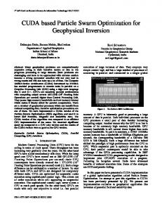
We offered an example of an EOL product that has 10 components and two tools with different drive sizes. Part 3 and Part 4 cannot be taken off by 2nd tool’s drive size. The structure of the EOL product is described in Fig. 1, and the detailed attributes for the disassembly components and tools are shown in Table II. TABLE II. Component k d(k) Tool i c(k) m(1,k) i=1 s(1,k) B(1,k) m(2,k) i=2 s(2,k) B(2,k)

1 +x S N 1 3 D 2 2

TABLE III. Sequence j Tool i Part k m(i,k) d(k) c(k) s(i,k) Bj(i,k) Tj(i) Dj(k) Mj(i,k) F(X)

1 1 2 N –x S 1 3 0 1 1

2 1 10 D +y A 0 2 0 1 0

INPUT DATA OF TDSP FOR EX. 1. 2 –x S N 1 3 N 1 2

3 +z S D 2 2

4 –z P N 1 3

5 –z P N 1 4 N 1 2

6 –y S D 2 2 D 0 1

7 –x P D 0 1 N 2 2

8 –z P N 1 3 D 0 2

9 +y A D 0 2 N 0 3

10 +y A D 0 2 N 0 3

THE FITNESS VALUE F(X) OF X={(I,K)J} 3 1 7 D –x P 0 1 1 2 0

4 2 (1 D +x (S (2 0 0 0 0

5 1 3 N +z S 2 0 0 0 0

6 1 6) D –y S) 2) 2 0 0 0

7 2 8 D –z P 0 2 0 0 1

8 2 5 N –z P 1 2 1 0 0

9 1 4 N –z P 1 3 0 1 1

10 1 9 D –y P 0 2

Total

17 2 5 3 27

disassembly precedence A1={1,2}; δ1={3,…,10} A2={7}; δ2={3,4,5,6} A3={6}; δ3={4,5} Fig. 1. Disassembly precedence relationship of the EOL product for Ex. 1 [6]

Table III shows a disassembly time (F(X)) of feasible solution X=((i=1,k=2)j=1, (1,10)2, (1,7)3, (2,1)4, (1,3)5, (1,6)6, (2,8)7, (2,5)8, (1,4)9, (1,9)10) when input data are given (Table II), and the feasible solution conforms to the rule of c(k),j=c(k),j+1 and s(i,k),j=s(i,k),j+1=2. Therefore, a block of components (1, 3, 6) could be disassembled simultaneously within 2 minutes and the disassembly time of parts 1 and 3 could be ignored. III.

SIMPLIFIED SWARM OPTIMIZATION

Simplified Swarm Optimization (SSO) [17], [23]-[25], a multi-role and population-based stochastic optimization technique, belongs to the category of Swarm Intelligence methods. In the quest for optimal TDSP, this paper proposes an advanced SSO (aSSO) which is a combination of the feasible solution generator (FSG), the self-adaptive parameter control (SPC), and the position updating procedure with the precedence preservative operator (PPO). A. Feasible Solution Generator Some solutions in the solution space are unfeasible as a result of the disassembly precedence constraints in the TDSP, but this paper presents a feasible solution generator that can produce a feasible solution set at once, avoiding the need to generate a new one or adjust an unfeasible solution. The proposed FSG is listed in Table IV. The concept of FSG is that if component α∈Ai must be disassembled prior to component set δi and the current available position is k, then the component α is randomly scheduled in a position from k to position (DIM-Card(δi)), where DIM is the total components and Card(δi) is the cardinality of posterior disassembled set δi. In accordance with the data given in Ex. 1 and the Procedure FSG, the initial solution is generated as follows. In Table IV, the first two subprocedures generate three precedent sets Ai=1,2,3, i.e. A1={1,2}, A2={7}, A3={6} and three decedent sets δi=1,2,3, i.e., δ1={3,…,10}, δ2={3,4,5,6}, δ3={4,5} (see Fig. 1). Components among three precedent sets are scheduled in sequence from 1 to r=3; other components within three decedent sets are then scheduled in reverse order from r=3 down to 1. Let component set Com={1,…,10} and position set Pos={1,…,10}. Regardless of the full- or partial-precedent set, a component from ith precedent set Ai will be extracted and reproduced as

2714

scheduled candidate A={2}, but if there are remainders in Ai, these remainders will be incorporated into ith decedent set (δ1=δ1∪(A1\{2})={1,3,…,10}). The scheduled candidate A (viz. component X(ki)) will be allocated to the position ki which randomly chooses from ki to (DIM-Card(δi)), i.e. ki∈{ki=1,…, DIM-Card(δ1)=10-9=1}. The next scheduled candidate A then starts in ki +1 and let Com and Pos subtract appointed X(ki) and ki, i.e. Com=Com-{2}={1,3,…,10}, Pos=Pos-{1}={2,3,…,10}. Similarly, the remaining precedent sets Ai are scheduled by the same process until maximal rule. By contrast, the decedent sets δi are scheduled from the end to the beginning. Initially, if rule index i is less than total rules r, prior decedent set δi requires subtracting elements in posterior decedent set δi+1, in which these components have already been assigned. Subsequently, the Ai’s position pos(Ai) must be orientated by means of sub-procedure, Find_Position(Ai). Behind the position pos(Ai), all components X(kj) among δi can be randomly assigned to the position kj from the rest of Pos included by the range {pos(Ai)+1,…, DIM}. Then, let Com and Pos subtract assigned X(kj) and kj. Similarly, the rest of the decedent sets δi are scheduled by the same process until the first rule index. TABLE IV.

PSUDOCODE OF FSG

Procedure Feasible_Solution_Generator Load_EOL_Product_Structure; Construct_Precedent_Rule; set Com={all components}; Pos={all positions}; ki:=1; for i:=1 to r do if Card(Ai) > 1 then A copies one element from Ai at random; Ai:= A; δi:= δi (Ai\A); else if Card(Ai)=1 then A:= Ai; end if ki selects one value from the range {ki,…, DIM－Card(δi)} at random; X (ki):=A; ki:= ki+1; let Com:= Com\{X (ki)}; Pos:= Pos\{ki}; next for for i:=r downto 1 do if i < r then {δi}:= {δi}\{δi+1}; end if pos(Ai):=Find_Position(Ai); for j:=1 to Card(δi) do select kj∈ Pos {pos(Ai)+1,…, DIM} at random; X (kj) equals jth element in {δi}; let Com:= Com\{X (kj)}; Pos:= Pos\{kj}; next for next for

{

}

{

}

FLB = ∑ k Min B(i,k ) (i,k ) ∉ S2 + Min B(i,k )(i,k ) ∈ S2 , i

{

}

where S2 = (i,k) s (i,k) =2

Notably, FLB assumes that in the same componential (ck) disassembly block, only the last component with minimal disassembly time B(i,k) needs to be considered, and the rest of the block must ignore the costs resulting from the penalty items for direction, method and tool changes because the disassembled blocks are disassembled together and used as material recovery (si,k=2). As in Ex. 1, S2={(i=2, k=1), (1, 3), (1, 6) | si,k=2}, and FLB = B(2, 2) + B(1, 4) + B(2, 5) + B(1, 7) + B(2, 8) + B(1, 9) + B(1, 10) + Min{B(2, 1), B(1, 3), B(1, 6)} = 16. We subsequently transform the original fitness values F(•) into the new fitness value F*(•) by means of formula (7), and define four ranges (viz. [0, Cw], [Cw, Cp], [Cp, Cg],and [Cg, 1]) as the probabilities of four particles (viz. gBest, pBest, current solution, random solution) be selected. Equations (7)-(12) show that the reciprocal is used to transform minimization into maximization, and the denominator magnifies the quality of a solution. Clearly, the F*(•) presents the quality of fitness value of a solution for producing the probability of a solution being selected (w.r.t. Cw, Cp, and Cg) [17]. Hence, these solutions with superior fitness values are likely to propagate their variable values to produce offspring. There are four roles (gBest, pBest, current solution, random solution) in SSO. At iteration t, gBest is the best-so-far solution G in the whole population, pBest is the best solution Pi, the current solution is Xi, and the random solution is a solution Xr generated at random. The following procedure describes the set-up of selection probability (viz. Cw, Cp, and Cg) in accordance with their new fitness value F*(•). F*(•) = [(F(•)-FLB) / F(•)]-1 *

*

*

t

*

(7)

Fi = F (Xi)+F (Pi)+F (G )+F (Xr)

(8)

Cg = 1-Max{cr=((F*(X) / Fi)), 0.2}

(9)

*

γ = Cg/(Fi- F (Xr)) *

Cw = γ × F (Xi) *

*

Cp = γ×( F (Xi)- F (Pi))

B. Self-Adaptive Parameter Control The more effective parameter values we set, the more efficient soft computing we achieve [6], [22]-[30], e.g., crossover and mutation rate in GA and three parameters of PSO. Their parameters play important roles in the exchange of information among solutions and so do the parameters of SSO [17], [23]-[25]. However, it is admittedly arduous and timeconsuming to specify adequate parameters for the optimization algorithms. In the SSO, the random values of Cw, Cp, and Cg in [0, 1] are related to the probability of the variable being selected from the current solution, gBest, and pBest [24]. The new solution comprises the selected variable values [17], [23][25]. In this section, a SPC is proposed to adjust Cw, Cp, and Cg, automatically. At the start of SPC, the lower bound of the disassembled time, FLB, is calculated using the following equation:

(6)

(10) (11) (12)

The proposed SPC (formula (7)-(12)) with the following PPO (formula (14)) provides the complete position updating procedure for the ith solution at iteration t+1 in the SSO. C. Position updating with Precedence Preservative Operator The sequence of components must follow the precedence relationship constraints. To avoid obtaining an infeasible solution for each particle in the search process, the PPO (Precedence Preservative Operator) is revised and integrated into the position updating procedure of SSO. The traditional PPO in a GA updates position according to two parents and produces two new solutions (chromosomes), whereas the revised PPO of the SSO updates position according to G, Pi, Xi, Xr and generates one new X. The PPO of SSO is depicted as follows:

2715

⎧ rand[0,1] , if rand[0,1]>0.5, or d=1 ρ dt = ⎨ t , otherwise ⎩ρ d-1 ⎧ L(X it-1 ) ⎪ t-1 ⎪ L(P ) X it (d)= ⎨ i t-1 ⎪ L(G ) ⎪ L(X tr ) ⎩

(13)

IV.

,if ρ dt ∈ [0,C w ) ,if ρ dt ∈ [C w ,C p ) ,if ρ dt ∈ [C p ,Cg )

(14)

,if ρ dt ∈ [Cg ,1)

where L(Xi), L(Pi), L(G) and L(Xr) are the values of the leftmost dimension in Xi, Pi, G and Xr respectively. When a solution updates each variable position by means of the revised PPO (formula 14), new solution Xi determines its selected roles grounded on four intervals ([0,Cw), [Cw,Cp), [Cp,Cg), [Cg,1)) to which the selected number ρd belongs. Notably, the selected number ρd is a uniform random number (viz. rand[0,1]). At times, the selected number ρd randomly makes consecutive dimensions learn from the same selected role in order to retain a useful portion of the disassembly sequence (formula (13)). In solution Xi, the updating operation of tool-variable tool_Xi(d) is identical to that of part-variable part_Xi(d) (formula 14). Xi Tool_Xi → Part_Xi →

d=1 Tool_Xi(1) Part_Xi(1)

d=2 Tool_Xi(2) Part_Xi(2)

…… ……

dimension. In sum, the pseudo code of the overall proposed SSO (integrating FSG, SPC, and PPO) is described in Table V. EXPERIMENTAL RESULTS AND COMPARISON STUDIES

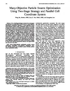
This section focuses on the quality and performance of the advanced SSO (aSSO) using five examples (Ex. 1-5). In the aforementioned TDSP of Ex. 1 [6], the EOL product consists of ten components and two available tools, whose disassembly precedence relationship is depicted in Fig. 1. Another EOL product comprises thirteen components whose fasteners can be disassembled by ten tools, and some fasteners cannot be taken off by some tools because of drive sizes and drive types. Accordingly, Ex. 2-5 are generated randomly, and their disassembly precedence relationship is illustrated in Fig. 3.

d=DIM Tool_Xi(DIM) Part_Xi(DIM)

Fig. 2. The phenotype of a solution (X2×DIM)

TABLE V.

PSUDOCODE OF ADVANCED SSO

Algorithm Simplified Swarm Optimization Read_TS-DSP_datum; Initialization_Populations(POP); (via FSG) repeat generate a Xrt; if (T(Xrt) < T(Gt)) then Xrt and Gt exchange each other; end if for i:=1 to POP do Self_adaptive_Parameter_Control (Xrt-1, Xit-1, Pit-1, Gt-1); Position_Updating_PPO(Xrt-1, Xit-1, Pit-1, Gt-1, Cw, Cp, Cg); Calculate_Fitness_Value(Xit); Find_pBest(T(Pit-1), T(Xit)); end for Find_gBest(T(Gt-1), T(Pit));

Fig. 3. Disassembly precedence relationship of the EOL product for Ex. 2-5.

until termination condition (e.g. maximum iterations or maximum time) is attained

In the TDSP, the solution Xi (Fig. 2) is a matrix X2×DIM including DIM parts and DIM tools, which are denoted as Tool_Xi and Part_Xi in ith solution Xi. In this regard, if a EOL product comprises 6 components and 2 tools, let the solution be a matrix [(Tool, Part)T]6, that is, 6 pairs of variables. Hence, Xi=[(1,1), (1,3), (2,4), (2,5), (1,6), (1,2)] = (11|13|24|25|16|12), Pi=(12|13|21|26|24|15), G=(21|22|23|16|14|15), Xr=(11|26|23| 22|15|24), Cw=0.3, Cp=0.6, and Cg=0.9. In the 1st dimension of new solution Xi, the selected number ρ1 is 0.2312∈[Cw=0.3, Cp=0.6)], so new Xi(1) selects the leftmost position from the current solution Xi(1), that is, tool_Xi(1)=1 and part_Xi(1)=1. The selected component will be disabled and cannot be selected again. In the 2nd dimension, the selected number ρ2 is 0.7594∈[Cp=0.6, Cg=0.9)], so part_Xi(2) similarly selects the leftmost dimension from the G(2); thus, tool_Xi(2) equals 2 and part_Xi(2) equals 2. Similarly, the remainder of new Xi(d) are scheduled by formulas (13) and (14) until maximal

There are two experiments in the work. The first focuses on analyzing the effects of the FSG and SPC, and the trade-off between populations and generations. The main point of the second experiment is to compare the aSSO with PPO-GA and PSO. In these experimental results, the subscripts, max, min, avg and std represent maximum, minimum, average, and standard deviation, respectively, obtained in 500 independent runs. The performance indices, F, G, and T signify the related fitness function value over 500 independent runs, the minimal number of generations that find the optimal or near-optimal solution in 500 independent runs, and the run time for each individual run, respectively. For instance, Fmin and Fmax are the minimal (best) and the maximal (worst) fitness function values in 500 independent runs. All methodologies are performed on an Intel Pentium 2.53 GHz PC with 4 GB memory. The operating system is MS Windows XP and the compiler is Visual Basic. A. Experiment 1: Statistical test of the advanced SSO There are disassembly precedence constraints in the TDSPs, so a number of redundant unfeasible solutions will be generated by the randKey of PSO and the randInt of PPO-GA [30]. In Fig. 4, we compare three initial solution generators, randKey, the randInt, and the proposed FSG, and the numeric result shows that the computational time of the randInt and randKey increases as the population size rises (POP=40–400); the performance of randInt is better than that of randKey, but the proposed FSG spends less than 1 ms on generating feasible solutions. While researchers experiment to obtain sufficient

2716

computational time (sec.)

observations, an algorithm requires setting big populations in a complex TDSP, performing a large number of running periods for the robust validation, or working out a specific nearoptimal or optimal solution for different EOL products. Thus, the proposed FSG will economize on the generation time of initial solutions for every algorithm and EOL product. 1.6 1.4 1.2 1 0.8 0.6 0.4 0.2 0

aSSO is satisfied in all cases, and in Ex.1 and Ex.3 especially, and the minimal convergent generation of the aSSO is effectual except for Ex.1-3. However, in terms of the running time, although the aSSO is less efficient than F1–F3, the worst ratio of Tavg in the case of aSSO and F1–F3 is 2.30:2.16=1:0.94, which is an acceptable trade-off between performance effectiveness and computational efficacy. In consequence, even though the proposed SPC slightly hinders the entire computational time for each individual run, it can assist the aSSO in solution quality and convergence speed, because the SPC automatically adapts and tunes cw, cp, and cg simultaneously, as long as fitness values throughout the entire search space provide the necessary momentum for a solution to move across the search space. Ex.2

40 80 120 160 200 240 280 320 360 400 randKey 0.063 0.234 0.406 0.531 0.719 0.891 1.031 1.203 1.406 1.531 randInt 0.016 0.063 0.141 0.203 0.266 0.3281 0.406 0.516 0.531 0.656 FSG 6.0E-06 1.1E-05 1.8E-05 3.2E-05 4.7E-05 7.2E-05 1.4E-04 2.6E-04 3.7E-04 3.9E-04

Fig. 4. Computational Time of the randKey, the randInt, the proposed FSG.

50

To demonstrate the power of the proposed SPC, four SSObased algorithms: advanced SSO and F1-F3 (the same as SSO but without SPC) are implemented. The three parameters, Cw, Cp, and Cg, are fixed in F1-F3. F1: Cw=.15, Cp=.40 and Cg=.75, which are adapted from the generic SSO [23]; F2: Cw=.10, Cp=.40 and Cg=.90, which are adapted from the published SSO [24]; F3: Cw=.10, Cp=.40 and Cg=.70. In these SSO-based algorithms, the condition of cw≤cp≤cg always holds, where cw=Cw, cp=Cp–Cw, cg=Cg–Cp, and cr=1–Cg. However, cr and cp are considered equally important in F1. Additionally, cg=.5 in F2 is larger than cg in F1 and F3, and cr=.30 in F3 is larger than cr in F1 and F2. Hence, F2 and F3 emphasize the role of gBest and random movements, respectively. TABLE VI.

Ex.

1

2

3

4

5

SSO F1 F2 F3 F1 F2 F3 F1 F2 F3 F1 F2 F3 F1 F2 F3

Ex.4

Ex.3

POP

13.4 13.3 13.2 13.1 13.0 12.9 12.8 12.7 12.6 12.5

POP

GEN

100

1000

2000

POP

GEN

16.0 15.9 15.8 15.7 15.6 15.5 15.4 15.3 15.2 15.1

GEN

20.1 20.0 19.9 19.8 19.7 19.6 19.5 19.4 50

100

1000

2000

50

100

1000

2000

Fig. 5. Main effect plot for POP and GEN in Ex. 2-4.

TABLE VII.

Ex. 1 2 3 4 5

STATISTICAL TEST FOR CASE1 AND CASE2 IN THE ASSO.

H0 : μcase1 = μcase2 vs. H1 : μcase1 ≠ μcase2 Convergent Fitness Value(F) Running Time(T) Generation(G) p-Value Superior p-Value Superior p-Value Superior 0.858 none 0 Case 1 0 Case 1 0 Case 1 0 Case 1 0 Case 1 0.004 Case 1 0 Case 1 0.274 none 0.036 none 0 Case 1 0 Case 1 0.780 none 0 Case 1 0 Case 1

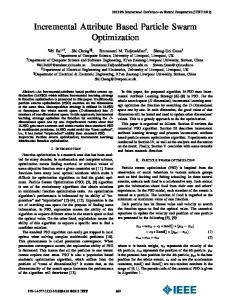
Due to the proposed SPC, there are only two essential parameters, i.e., POP and GEN, in the advanced SSO (aSSO). This paper has a factorial design experiment of two factors with two levels, i.e., POP=50 or 100, GEN=1000 or 2000. According to the experimental results of factorial design (Fig. 5), the two main effects and their interaction have a splendid influence on the outperformance of aSSO in the TDSPs; however, the increment of the generation’s level is less efficient than that of the population’s level with reference to the main effects for Ex. 2-4. This paper selects two special cases, i.e., Case1: (POP=100, GEN=1000) and Case2: (POP=50, GEN=2000) within the same calculation frequency of fitness function to compare the performance of aSSO with an increment of POP and of GEN. As a result (Table VII), the performance of Case 1 is better than that of Case 2, whatever the fitness value, convergent generation or running time may be. Hence, this paper suggests that the population number should be increased first when the aSSO is applied to various and complex TDSPs.

PAIRED T-TEST RESULTS FOR SSO (F1–F3) AND ASSO. H0 : μaSSO = μcompetition vs. H1 : μaSSO ≠ μcompetition Convergent Fitness Value(F) Running Time(T) Generation(G) p-Value Superior p-Value Superior p-Value Superior 0.685 none 0.190 none 0 F1 0 aSSO 0 F2 0 F2 0.652 none 0.781 none 0 F3 0.909 none 0.571 none 0 F1 0.185 none 0 F2 0 F2 0.843 none 0.107 none 0 F3 0.844 none 0.611 none 0 F1 0.060 none 0 F2 0 F2 0.001 aSSO 0.364 none 0 F3 0.110 none 0 aSSO 0 F1 0.135 none 0.175 none 0 F2 1 none 0 aSSO 0 F3 0.521 none 0 aSSO 0 F1 0.854 none 0.175 none 0 F2 0.206 none 0 aSSO 0 F3

The quality of parameter design affects the performance of algorithms; therefore, we suppose that the advanced SSO (aSSO) attached to the proposed SPC could adequately dispose of general TDSPs. On the basis of the experimental result and statistical analysis (Table VI), the fitness function value of the

B. Experiment 2: Comparison of the aSSO with PPO-GA and PSO In this experiment, the advanced SSO (aSSO), the PPO-GA and the PSO are compared fairly by statistic test for two special settings in consideration of the same calculation frequency of

2717

fitness function. Case 1 specifies population of 100 individuals with 1000 generations, and Case 2 specifies population of 50 individuals with 2000 generations. TABLE VIII. Case 1 Ex. 1 2 3 4 5

Alg. PPO-GA PSO PPO-GA PSO PPO-GA PSO PPO-GA PSO PPO-GA PSO

TABLE IX.

PSO. The experimental result has proved that the proposed aSSO with sufficient populations is adequate for addressing numerous complicated TDSPs. V.

STATISTIC TEST FOR ASSO AND COMPETITION IN CASE 1.

CONCLUSIONS AND FUTURE WORKS

In general, a disassembly task should be implemented by finite specialized tools. Consequently, providing adequate tools is necessary for accelerating disassembly, and filtering redundant tools is beneficial for each disassembly factory. Accordingly, the proposed TDSP is a useful and realistic model for the recycling issue of EOL product, and solution procedure of TDSP should be fully investigated. The proposed solution procedure, in which aSSO is combined from FSG, SPC, and PPO, is devoted to the optimization of TDSP for a given EOL product. As discussed in the statistical analysis in Section IV, the FSG reduces the computational time in initialization, the SPC navigates each solution to a superior evolutional direction without regard to factorial design except for population and generation, and the position updating procedure conserves the solution’s validity by using the revised PPO for efficacious evolution. Therefore, the computational efficacy and performance effectiveness in the proposed aSSO are better than they are in PPO-GA and PSO. As a result, the proposed aSSO guarantees efficiency in identifying the optimum disassembly sequencing and tool assignment in a TDSP.

H0 : μaSSO = μAlg. vs. H1 : μaSSO ≠ μAlg. Convergent Fitness Value(F) Running Time(T) Generation(G) p-Value Superior p-Value Superior p-Value Superior 0 aSSO 0 PPO-GA 0 aSSO 0 aSSO 0 PSO 0 aSSO 0 aSSO 0 PPO-GA 0 PPO-GA 0 aSSO 0 PSO 0 aSSO 0 aSSO 0 PPO-GA 0 PPO-GA 0 aSSO 0 PSO 0 aSSO 0.028 none 0 PPO-GA 0 aSSO 0 aSSO 0 PSO 0 aSSO 0 aSSO 0 PPO-GA 0 aSSO 0 aSSO 0 PSO 0 aSSO STATISTIC TEST FOR ASSO AND COMPETITION IN CASE 2.

H0 : μaSSO = μAlg. vs. H1 : μaSSO ≠ μAlg. Convergent Running Time(T) Generation(G) Ex. Alg. p-Value Superior p-Value Superior p-Value Superior PPO-GA 0 aSSO 0 PPO-GA 0 PPO-GA 1 PSO 0 aSSO 0 PSO 0 aSSO PPO-GA 0 aSSO 0 PPO-GA 0 PPO-GA 2 PSO 0 aSSO 0 PSO 0 aSSO PPO-GA 0 aSSO 0 PPO-GA 0 PPO-GA 3 PSO 0 aSSO 0 PSO 0 aSSO PPO-GA 0 aSSO 0 PPO-GA 0 PPO-GA 4 PSO 0 aSSO 0 PSO 0 aSSO PPO-GA 0 aSSO 0 PPO-GA 0 PPO-GA 5 PSO 0 aSSO 0 PSO 0 aSSO Case 2

Fitness Value(F)

According to Tables VIII and IX, the aSSO almost outperforms the PPO-GA and PSO in terms of fitness value (F), except for Ex. 4 in Case 1. Although the aSSO is worse than the PPO-GA and PSO in respect of the convergent generation (G), the aSSO postpones converging on the population evolution to explore unknown solution space and exploit a near-optimal or optimal solution. However, an interesting observation is that Case 1 and Case 2 in the running time (T) have distinct consequences. The aSSO in Case 1 is mostly more efficient than the PPO-GA and PSO, but in Case 2 it is better than the PSO and less efficient than the PPO-GA. As far as the solution’s validity is concerned, on the strength of the proposed FSG and the revised PPO, the aSSO avoids generating unfeasible solutions in initialization and evolutionary procedures, the PPO-GA applies the precedence preservative crossover to ensure evolutionary solutions are feasible, but the PSO utilizes the disassembly precedence constraints alone to restrain all evolutionary procedures from generating infeasible solutions. Thus, the different computational efficacy for aSSO and PPO-GA in the two special cases is that the population number in Case 1 is twice as big as that in Case 2, so the PPO-GA of Case 1 has more chance of generating infeasible solutions in the mutation operation. Consequently, the PPO-GA with big populations spends more time excluding infeasible solutions, as does the

Future work will ameliorate aSSO by integrating another powerful local search technique to solve other, more complex combinatorial optimization problems, and by analyzing the interactive effect of four selected roles (gBest, pBest, current solution, and random solution) to verify the performance of these combination algorithms. Furthermore, the proposed TDSP model might be studied from the aspect of the disassembly tool’s utilization, recycling cost, or other practical viewpoints. REFERENCES [1]

[2]

[3]

[4]

[5]

[6]

[7]

2718

S.M. Gupta and S.M. McGovern, Multi-objective optimization in disassembly sequencing problems, Second World Conference on POM and 15th Annual POM Conference, Cancun, Mexico, April 30 - May 3, 2004. J. Pomares, F. A. Candelas, et al, Safe human-robot cooperation based on an adaptive time-independent image path tracker, International Journal of Innovative Computing Information and Control, vol. 6, no. 9, pp. 3819-3842, 2010. A. Gungor, M. Surendra, and S.M. Gupta, Disassembly sequence plan generation using branch-and-bound algorithm, International Journal of Production Research, vol. 39, no. 3, pp. 481-509, 2001. S.M. McGovern and S.M. Gupta, Ant colony optimization for disassembly sequencing with multiple objectives, International Journal of Advanced Manufacturing Technology, vol. 30, no. 5-6, pp. 481-496, 2006. A.J.D. Lambert and S.M. Gupta SM, Disassembly Modeling for Assembly, Maintenance, Reuse, and Recycling, CRC Press, Boca Raton, Florida, 2005. E. Kongar and S.M. Gupta, Disassembly sequencing using genetic algorithm, The International Journal of Advanced Manufacturing Technology, vol. 30, no. 5-6, pp. 497-506, 2006. V.N. Rajan and S.Y. Nof, Minimal precedence constraints for integrated assembly and execution planning, IEEE Transactions on Robotics and Automation, vol. 12, no. 2, pp.175-186, 1996.

[8]

[9]

[10]

[11]

[12]

[13]

[14]

[15]

[16]

[17]

[18]

Z. H. Che, Using hybrid genetic algorithms for multi-period product configuration change planning, International Journal of Innovative Computing Information and Control, vol. 6, no. 6, pp. 2761-2785, 2010. Y. Tang, M. Zhou, and M. Gao, Fuzzy-Petri-Net-based disassembly planning considering human factors, IEEE Transactions on Systems, Man and Cybernetics, Part A: Systems and Humans, vol. 36, no. 4, pp. 718-726, 2006. S.M. Gupta and S.M. McGovern, Greedy algorithm for disassembly line scheduling, IEEE International Conference on Systems, Man and Cybernetics, vol. 2, no. 5-8, pp. 1737–1744, 2003. K.-M. Lee and M. Bailey-Van Kuren, Modeling and supervisory control of a disassembly automation workcell based on blocking topology, IEEE Transactions on Robotics and Automation, vol. 16, no. 1, pp.67-77, 2000. Y. Tang, M.C. Zhou, and R. Caudill, An integrated approach to disassembly planning and demanufacturing operation, IEEE Transactions on Robotics and Automation, vol. 17, no. 6, pp. 773-784, 2001. S.M. Mok, C.-H. Wu, and D.T. Lee, Modeling automatic assembly and disassembly operations for virtual manufacturing, IEEE Transactions on Systems, Man and Cybernetics, Part A: Systems and Humans, vol. 31, no. 3, pp. 223-232, 2001. M.M. Gao, M.C. Zhou, and R. Caudill, Integration of disassembly leveling and bin assignment for demanufacturing automation, IEEE Transactions on Robotics and Automation, vol. 18, no. 6, pp. 867-874, 2002. S.C. Sarin, H.D. Sherali, and A. Bhootra, A precedence-constrained asymmetric traveling salesman model for disassembly optimization, IIE Transactions, vol. 38, no. 3, pp. 223-237, 2006. A.J.D. Lambert and S.M. Gupta, Methods for optimum and near optimum disassembly sequencing, International Journal of Production Research, vol. 46, no.11, pp. 2845-2865, 2008. W.C. Yeh, Optimization of the disassembly sequencing problem on the basis of self-adaptive simplified swarm optimization, IEEE Transactions on Systems, Man and Cybernetics-Part A: Systems and Humans, vol. 42, no. 1, pp. 250-261, 2011. E. Zussman, A. Krivet, and G. Seliger, Disassembly oriented assessment methodology to support design for recycling, CIRP Annals Manufacturing Technology, vol. 34, no.1, pp.9-14, 1994.

[19] J.-H. Lin, R.W. McGorry, P.G. Dempsey, and C.-C. Chang, Handle displacement and operator responses to pneumatic nutrunner torque buildup, Applied Ergonomics, vol. 37, no. 3, pp. 367-376, 2006. [20] C. Chung and Q. Peng, Tool selection-embedded optimal assembly planning in a dynamic manufacturing environment, Computer-Aided Design, vol. 41, no. 7, pp. 501-512, 2009. [21] C. Bierwirth, D.C. Mattfeld, and H. Kopfer, On permutation representations for scheduling problems, Parallel Problem Solving from Nature IV, eds. H.-M. Voigt, W. Ebeling, I. Rechenberg and H.-P. Schwefel, Springer, Berlin, pp. 310-318, 1996. [22] C. Bierwirth, D.C. Mattfeld, Production scheduling and rescheduling with genetic algorithms, Evolutionary Computation, vol.7, no.1, pp. 117, 1999. [23] W. C. Yeh, W. W. Chang and C. W. Chiu, A simplified swarm optimization for discovering the classification rule using microarray data of breast cancer, International Journal of Innovative Computing, Information and Control, vol. 7, no. 5, pp. 2235-2246, 2011. [24] W.C. Yeh, A two-stage discrete particle swarm optimization for the problem of multiple multi-level redundancy allocation in series systems, Expert Systems with Applications, vol. 36, no. 5, pp. 9192-9200, 2009. [25] W.C. Yeh, Simplified swarm optimization in disassembly sequencing problems with learning effects, Computers & Operations Research, vol. 39, no. 9, pp. 2168-2177, 2012. [26] J. Kennedy and R.C. Eberhart, Neural networks: Particle swarm optimization, Proceedings of the IEEE International Conference, vol. 27, pp. 1942-1948, 1995. [27] J. Kennedy and R.C. Eberhart, A discrete binary version of the particle swarm algorithm, Proceedings of IEEE International Conference on Systems, Man and Cybernetics, Oct. 12-15, vol. 5, pp. 4104-4108, 1997. [28] Y. Shi and R.C. Eberhart, Evolutionary computation: Empirical study of particle swarm optimization, Proceedings of the 1999 Congress, on Evolutionary Computation, pp. 1945-1950, 1999. [29] J. Kennedy, R.C. Eberhart, and Y. Shi, Swarm Intelligence, Morgan Kaufmann, New York, 2001. [30] J.C. Bean, Genetic algorithms and random keys for sequencing and optimization, ORSA Journal on Computing, vol. 6, no. 2, pp. 154-160, 1994.

2719