Smooth Penumbra Transitions with. Shadow Maps. WILLEM H. DE BOER. Playlogic Game Factory B.V. 1. We present a method for rendering aesthetically ...
Smooth Penumbra Transitions with Shadow Maps WILLEM H. DE BOER Playlogic Game Factory B.V.
1
We present a method for rendering aesthetically correct soft shadows that exhibit smooth inner and outer penumbrae and self-shadowing. Our approach is an extension of ordinary shadow mapping; in an additional step, occluder shadow silhouette edges, as seen from the center of an area light, are detected and extruded into so-called Skirts. This step is done entirely in image space, and as such does not require the construction of extra geometric primitives. During final rendering, penumbra regions are identified using the depth information of the Skirts and stochastic sampling of the shadow map. Our algorithm has been successfully implemented on programmable shader hardware, and interactive framerates are obtained. We observe that the main bottleneck of our implementation lies in the rasterisation stage; performance mainly depends on the size of the lightsource. Categories and Subject Descriptors: I.3.7 [Computer Graphics]: Three-dimensional graphics and realism General Terms: Algorithms, human factors, performance Additional Key Words and Phrases: Hardware accelerated image synthesis, illumination, image processing, shadows
1
1.
INTRODUCTION
Real-time soft shadow techniques have received a lot of attention by the graphics research community. Recent advances in graphics hardware have made it possible to extend existing hard shadow algorithms ([Williams 1978] and [Crow 1977]) to render soft shadows at interactive or real-time framerates. Most of these methods rely on object space techniques for extracting an occluder’s shadow silhouette edges. These edges are essential to identifying penumbra regions, as we shall discuss later. Unfortunately, the performance of these object space approaches depends on the geometric complexity of the scene. In this paper, we are interested in modifying Williams’ shadow map algorithm to incorporate aesthetically correct soft shadows. More specifically, we are looking for an algorithm that (1) has a constant and controllable time complexity, independent of the complexity of the scene in terms of the number of primitives used (e.g. triangles, surface patches); (2) does not exhibit any ”banding” or other quantisation artifacts of soft shadow boundaries, and (3) it must incorporate the ”softening” effect of the shadow over distance. 1 The
author has since left the company, and now works for Microsoft Research in Cambridge, United Kingdom
2
·
Submitted to the Journal of Graphics Tools
Fig. 1.
A simple concave object casts a shadow on a plane.
As will become clear later, the last point is equivalent to being able to distinguish between so-called ”inner” penumbrae and ”outer” penumbrae. Many soft shadow algorithms construct explicit representations of penumbrae, by extending shadow silhouette edges outwards in light space [Chan and Durand 2003] [Wyman and Hansen 2003] [Haines 2001] using geometric primitives. We will also build explicit penumbra representations, but in contrast to other approaches we will (i) construct these in image space, and (ii) build them in a way that allows us to render both inner penumbrae as well as outer penumbrae. 2. 2.1
SMOOTH PENUMBRA TRANSITIONS Preliminaries
Consider Figure 1, which is a cross section of a very simple scene consisting of one occluder and a receiver. We see that edge e1 on the right casts a hard shadow boundary onto the receiver. This edge is a silhouette edge as seen from the centre of the area lightsource; it is shared by two faces, only one of which is facing the light. Edge e2 is also a silhouette edge, however, it does not cast a shadow boundary. The main observation is that shadow boundaries are cast only by those silhouette edges, such as e1 , for which the dihedral angle is bigger than π radians. We will refer to such edges as shadow silhouette edges. Note that with this construction, the edge below and to the left of e2 is a silhouette edge, and its dihedral angle implies that it should also cast a shadow. However, because it lies in shadow itself it will not be classified as such. For area lightsources, shadow boundaries are not hard, but rather they are ”spread out” to a penumbra region. (From hereonafter, when we refer to an area
Smooth Penumbra Transitions
(a)
·
3
(b)
Fig. 2. (a) Three silhouette edges and a Skirt belonging to one (top view). (b) Calculating a point’s visibility value (side view). The thick black line represents a sideview of a Skirt.
lightsource, we will mean a disk-shaped lightsource with radius, r.) We will distinguish between two types of penumbra regions: the outer penumbra, which separates the completely lit region from the hard shadow boundary; and the inner penumbra which separates the umbra from the hard shadow boundary. We also note that the inner penumbra is situated where an umbra would have been, had the scene been lit by a point lightsource. As the inner penumbra increases in size (with an increase in distance between receiver and occluder) the umbra decreases in size accordingly. This gives rise to the ”softening” effect of the cast shadow the further a receiver is removed from its occluder. 2.2
Introducing shadow skirts
As has been shown by other researchers, it is possible to construct special ”primitives” that help us to detect penumbra regions; smoothies and the cones and sheets of penumbra maps [Chan and Durand 2003] [Wyman and Hansen 2003] are examples of primitives that have been used in the past. In contrast to these approaches, we construct our primitives using image processing techniques. Nevertheless, they still have a very intuitive geometric interpretation: Figure 2 a illustrates our penumbra or Skirt, for a single shadow silhouette edge; each shadow silhouette edge is associated with a unique Skirt. We note that a Skirt has the following three properties: (1) Its width is fixed to twice the radius of the lightsource;
4
·
Submitted to the Journal of Graphics Tools
Fig. 3. The 3 × 3 construction filter. Note how the centre entry is 0; we explicitly add the corresponding texel value to the filter sum, which guarantees us that shadow silhouette edges always have the value 1.
(2) it has a grey value, α, which is 1 (i.e. maximum intensity) at its associated shadow silhouette edge, and which fades to 0 (i.e. minimum intensity) towards both its lateral edges; (3) it contains depth information. Figure 2 b shows how to calculate the shadow value of a point in the penumbra region. Such a point, p, is ”occluded” by a Skirt, and must therefore lie in a penumbra region. We calculate p’s visibility value V (p) ∈ [0, 1] as follows: V (p) =
1 αs ( + 1) 2 (1 − zz10 )
(1)
where αs ∈ [−1, 1] is the transformed grey value, α, of the Skirt corresponding to p: � αs =
(α − 1) if p is in shadow, (1 − α) otherwise.
(2)
Note that Eq. (1) incorporates the ratio of distances between receiver, occluder, and lightsource. This is done for the same reason as with smoothies [Chan and Durand 2003], and allows us to calculate the correct penumbra size for any point on the receiver. It is important to note that with this construction, in image space, penumbra regions can never be wider than the width of a Skirt. 3. 3.1
ALGORITHM Constructing the Skirts
Before we can construct Skirts, we need to find all shadow silhouette edges in the scene. A very useful property of a shadow silhouette edge is that – for nonintersecting geometry – it is a line of discontinuity in the shadow map [McCool 2000]. Therefore, by applying an edge-detection filter to the shadow map we can identify all shadow silhouette edges. We store these edges with a grey value of 1 in an otherwise black Skirt buffer. We then construct the Skirts by iteratively applying a special 3 × 3 filter to this buffer. Figure 3 illustrates the entries of the filter kernel. With each iteration, we widen every Skirt in the buffer by 1 shadow map texel in all directions. We perform as many iterations as the radius of the
Smooth Penumbra Transitions
·
5
Fig. 4. An example of a shadow map (left), its shadow silhouette edges (middle), and the associated final Skirts buffer (right).
Fig. 5.
A case where point p is incorrectly classified as lying in an inner penumbra.
lightsource, r. Figure 4 shows examples of the different maps used in the Skirt creation process. The following procedure outlines the filter algorithm for a single texel, t. ConstructSkirt( texel t, lightradius r ) b