Finally, we show how warping and partitioning can be combined for interactive rendering of low error shadows in scenes with a high depth range. Categories ...
Eurographics Symposium on Rendering (2006) Tomas Akenine-Möller and Wolfgang Heidrich (Editors)
Warping and Partitioning for Low Error Shadow Maps D. Brandon Lloyd, David Tuft, Sung-eui Yoon, and Dinesh Manocha University of North Carolina at Chapel Hill http://gamma.cs.unc.edu/wnp /
Figure 1: These 800 × 800 resolution images show the benefit of combining shadow map warping and frustum partitioning algorithms on a power plant model with a high depth range. Left: A 2K × 2K shadow map generated with only a warping algorithm (LSPSM) has high aliasing error concentrated near the viewer. Middle: A 4K × 4K shadow map (the largest possible on current GPUs) still shows severe aliasing. Right: Warping combined with four frustum partitions produces low aliasing error using a total resolution of 2K × 2K while showing only a 30% drop in frame rate. The aliasing error is distributed more uniformly over the scene.
Abstract We evaluate several shadow map algorithms based on warping and partitioning using the maximum perspective aliasing error over the entire view frustum. With respect to our error metric, we show that a range of warping parameters corresponding to several previous warping algorithms have the same error. We also analyze several partitioning schemes to determine which produces the least maximum error using the least number of partitions. Finally, we show how warping and partitioning can be combined for interactive rendering of low error shadows in scenes with a high depth range. Categories and Subject Descriptors (according to ACM CCS): I.3.7 [Computer Graphics]: Three-Dimensional Graphics and Realism – Color, Shading, Shadowing and Texture
1. Introduction Shadows are an important component of an interactive rendering system. Shadow maps are one popular technique for rendering shadows. The standard shadow map algorithm as proposed by Williams [Wil78] is a two pass algorithm that first creates a depth map by rendering the scene from the light’s view. In the second pass, the depth map is used to determine which surfaces lie in shadow. Shadow maps are a particularly attractive algorithm because they are easy to imc The Eurographics Association 2006.
plement, they support a wide variety of geometry representations, and there exists wide support for shadow maps in current graphics hardware. The main drawback of shadow maps is aliasing errors at shadow edges. Aliasing occurs when the local sampling density in the shadow map is too low. The aliasing errors are worst for scenes with a high depth range because samples in the shadow map must cover larger regions. Two main approaches are used to address the sampling
B. Lloyd, D. Tuft, S. Yoon, & D. Manocha / Warping and Partitioning for Low Error Shadow Maps
problem: warping and partitioning. Warping algorithms render a reparameterized shadow map that leads to increased sampling resolution where it is needed [SD02, WSP04, MT04, CG04]. Since warping algorithms simply change the 4 × 4 matrix used to render a standard shadow map, they incur almost no performance penalty and can be easily implemented on current GPUs. Partitioning algorithms take a different approach. These algorithms partition the scene and use a separate shadow map for each partition [TQJN99, FFBG01, Arv04, LKS∗ 06]. For example, one shadow map may be used for areas close to the viewer and another for the rest of the scene. While partitioning can reduce aliasing error, rendering shadow maps for too many partitions may be expensive. Some algorithms combine warping and partitioning [Koz04, CG04]. It is often difficult to determine which algorithm is best for a given situation. Moreover, it is not clear how and when to switch between different techniques. We seek a single shadow map algorithm that has low aliasing error and maintains high performance for complex models with high depth range. Main Results: In this paper we present an error metric for evaluating shadow map algorithms based on the maximum perspective aliasing error over the entire view frustum. Aliasing error can be decomposed into two parts [SD02]: perspective aliasing, which depends only on the position of the light relative to the camera, and projection aliasing, which depends on the orientation of surfaces in the scene. We base our error metric on perspective aliasing because it is scene independent. Though we deal only with directional light sources in this paper, the error metric analysis can be extended to point lights. Using our error metric we investigate how to combine warping and partitioning to obtain a low error shadow map solution with good performance and guarantees on the aliasing error. Warping algorithms based on perspective projections, such as perspective shadow maps (PSMs) [SD02], light-space perspective shadow maps (LSPSMs) [WSP04], and trapezoidal shadow maps (TSMs) [MT04] differ primarily in the way the perspective parameter is chosen. We show that when the aliasing errors in both shadow map dimensions are combined, the total error for a range of parameter values is the same. The equivalent parameter range corresponds to these algorithms. We also consider two kinds of view frustum partitioning: • Face partitioning splits the view frustum at the edges of its faces as seen from the light’s point of view. Face partitioning allows warping to be used when it could not be used otherwise (e.g. when the light direction is parallel to the view direction) leading to reduced error. • z-partitioning subdivides the view frustum or its face partitions along their length. z- partitioning provides error reductions for all light directions. Frustum partitioning and z-partitioning can also be com-
bined. We show that for a given number of partitions, zpartitioning combined with warping delivers the least maximum error over the entire view frustum. We demonstrate the performance of this hybrid algorithm on a small model, typical of a game-like environment, and on massive models rendered by a view-dependent rendering algorithm. The rest of this paper is organized as follows. In Section 2 we briefly discuss work related to shadow map computation. In Section 3, we discuss how aliasing error should be measured and justify our choice of error metric. We analyze shadow map warping algorithms in Section 4 and frustum partitioning schemes in Section 5. We describe various implementation details for partitioned shadow maps in Section 6. In Section 7, we show some experimental results for combinations of partitioning and warping that lead to low aliasing error. Finally, we conclude with some ideas for future work. 2. Previous Work Many techniques have been proposed for shadow generation. In this section, we limit ourselves to shadow maps and some hybrid combinations with object-space techniques. Shadow maps were first introduced by Williams [Wil78]. Segal et al. [SKv∗ 92] later implemented them on standard graphics hardware. In order to hide shadow map aliasing, Reeves et al. [RSC87] filtered depth values to blur shadow map edges. Recently Donnelly and Lauritzen [DL06] introduced a way to use depth variance to facilitate better filtering of shadow depth maps. Other algorithms seek to remove aliasing by locally increasing the shadow map resolution where it is needed, either through warping or partitioning, or both: • Partitioning algorithms. Tadamura et al. [TQJN99] use z-partitioning for rendering scenes illuminated with sunlight. Adaptive shadow maps [FFBG01] use a quadtree that is refined in areas with high aliasing error. Increased programmability of GPUs has facilitated implementations of adaptive shadow maps for hardware rendering [LKS∗ 06], but performance can be slow. Tiled shadow maps [Arv04] partition a shadow map into tiles of different sizes guided by an aliasing measurement heuristic. • Warping algorithms. Shadow map warping was introduced with perspective shadow maps (PSMs) [SD02]. PSMs use the camera’s perspective transform to warp the shadow map. A singularity may arise with PSMs that requires special handling [Koz04]. Light-space perspective shadow maps (LSPSMs) [WSP04] are a generalization of PSMs that do not have the singularity problem because they use a perspective projection that is oriented perpendicular to the light direction. Trapezoidal shadow maps (TSMs) [MT04] are similar to LSPSMs, except that they use a different formulation for the perspective parameter. • Combined algorithms. Chong and Gortler [CG04] use a general projective transform to ensure that there is a oneto-one correspondence between pixels in the image and c The Eurographics Association 2006.
B. Lloyd, D. Tuft, S. Yoon, & D. Manocha / Warping and Partitioning for Low Error Shadow Maps
w'l
light beam
wl w'i
w'i
w'i
l
image beam
i
wi
w'i w'l
Figure 1: Shadow map aliasing. An image beam through a pixel and a light beam through a shadow map texel project onto a surface (left). When the light beam footprint is larger than the image beam footprint (upper-right), the light beam footprints can be distinguished as a jagged shadow edge (lower-right). the texels in the shadow map on a single plane within the scene. They use a small number of shadow maps to cover a few large surfaces. Kozlov [Koz04] proposed using a cube map in the post-perspective space of the camera. This corresponds to combining warping with face partitioning. Irregular shadow maps [JMB04, AL04] avoid the aliasing problem altogether by storing shadow map samples that correspond exactly to the image samples for the eye. However, irregular shadow maps are difficult to implement on current graphics hardware. Pure object-space shadow algorithms, such as shadow volumes, do not have aliasing problems. Some hybrid algorithms combine object-space techniques with shadow maps to reduce aliasing. McCool et al. [McC00] construct shadow volumes from a shadow map. Sen et al. [SCH03] create a shadow map that more accurately represents shadow edges. Both of these techniques, while generating better looking shadow edges, may miss small features if the shadow map resolution is inadequate. Chan and Durand [CD04] use shadow maps to restrict shadow volume rendering to the shadow edges. Govindaraju et al. [GLY∗ 03] use shadow polygons for the most aliased areas and a shadow map everywhere else. 3. Measuring aliasing error This section provides an overview of shadow map aliasing and introduces our error metric. We first review how shadow map aliasing occurs. Then we justify why we ignore projection aliasing and discuss the use of maximum perspective aliasing error over the whole frustum for evaluating shadow map algorithms. 3.1. Shadow map aliasing Figure 1 offers geometric intuition of how shadow map aliasing occurs. A beam emanates from the eye through a pixel on c The Eurographics Association 2006.
the image plane and projects onto a surface in the scene with a footprint of width w′i at the intersection point. A beam from the light through a shadow map texel projects onto the same location with a footprint of width w′l . When w′l > w′i , the light beam footprint is covered by multiple image beams and becomes distinguishable as a jagged, aliased edge at shadow boundaries. Following Stamminger and Drettakis [SD02], the aliasing error can be quantified as the mismatch ratio of the beam footprint widths: m=
w′l w cos θi ≈ l , w′i wi cos θl
(1)
where wi and wl are the widths of the image and light beams at the point of intersection and θi and θl are the angles between the surface normal and the beam directions. The wl /wi term is referred to as perspective aliasing. Perspective aliasing depends solely on the relative positions of the light and camera. It is independent of the scene geometry. The cos θi / cos θl term is referred to as projection aliasing. This term depends on the orientation of the surfaces in the scene relative to the camera and the light. Perspective aliasing vanishes when the beam widths are the same, i.e. wi = wl . Projection aliasing vanishes when the surface is oriented with its normal parallel or perpendicular to the half-way vector between the beam directions, i.e. θi = θl . 3.2. Ignoring projection aliasing Ideally, a shadow map algorithm should ensure that m = 1 everywhere in the scene. When m > 1 shadow map aliasing can appear at shadow boundaries. When m < 1, no aliasing appears, but the shadow map is oversampled and resolution is wasted. In practice, an ideal shadow map is difficult to compute due to the projection aliasing factor. Because of projection aliasing, the local resolution needed for different parts of the scene may vary dramatically depending on the orientations of the surfaces in the scene. Computing the resolution needed for each part of the scene requires a potentially expensive scene analysis, and storing an ideal shadow map requires data structures more complex than a regular grid. Adaptive shadow maps (ASMs) approach the ideal by storing the shadow map in a quad-tree and refining where more resolution is needed. But on current hardware, ASMs are too slow to provide all but a fairly coarse level of subdivision at high frame rates in a complex environment. Chong et al. [CG04] compute an optimal shadow map for a few surfaces in the scene, but for other surfaces there are no guarantees on the aliasing error. We choose to ignore projection aliasing and to minimize perspective aliasing. This means that we can use a shadow map parameterization that is both independent of scene complexity and is simple and efficient to compute. In practice, projection aliasing error might not ever be completely eliminated because it is potentially unbounded. However if perspective aliasing error is small, the projection aliasing that
B. Lloyd, D. Tuft, S. Yoon, & D. Manocha / Warping and Partitioning for Low Error Shadow Maps
light direction
t
0 shadow plane warping frustum
1
wi
eye
c
wl y view frustum
z
Figure 2: Visualizing aliasing error. These images show shadow map texels projected onto a scene consisting of a simple ground plane and an overhead directional light. The LSPSM algorithm (left) appears to be inferior to the PSM algorithm (right) due to projection effects. To see perspective aliasing more clearly, a plane is inserted on the left side of each image into the area of maximum perspective aliasing for each algorithm and is oriented such that projection effects are mostly removed. LSPSMs show error distributed evenly in both directions, while the error for PSMs is concentrated in a single direction. Both images, in fact, have the same total error. does remain is much less visible for at least two reasons First, when projection aliasing stretches light beam footprints across a surface, the sampling resolution is reduced only in the stretched direction. Second, surfaces which exhibit high projection aliasing error are nearly parallel to the light. For many surfaces, when the light angle is low, little light is reflected, so the shadows are not as noticeable anyway. 3.3. Maximum perspective aliasing error For our error metric we minimize the L∞ norm of perspective aliasing error. Specifically, we seek to minimize the maximum value the wl /wi term of m in Eq. (1) over the entire view frustum. Other norms could be used such as the L1 or the L2 norms. These norms tend to ensure that the "average" error is low, but high error outliers may occur. (For a more in-depth discussion of error measures in the context of shadow map rendering see [Cho03].) For specific views, where there are no surfaces or shadows in an area with high error, it may be possible for one shadow map to appear to have lower error than another, even if quantitatively it is inferior (see Figure 2). But in an interactive application where the view is unconstrained or the scene geometry is arbitrary, there is no guarantee that the "bad areas" will not become visible. Our metric gives guarantees on the worst case error independent of the scene. 4. Shadow map warping with perspective projections Perspective projections are used by prior warping techniques to reduce aliasing. The aliasing error is affected by both the warping parameter and the dimensions of the shadow map
0 0
n
z
f
n'
z'
f'
Figure 3: Perspective projection parameterization. Light space is defined with the y-axis aligned with the light direction, and the z-axis in the plane of the y-axis and view direction. The t-axis of the shadow map is aligned with the z-axis. The x and s axes point out of the page. The shadow map is warped by placing a warping frustum along the z-axis around the view frustum. The warp is controlled by varying the parameter n′ . relative to the image. In this section, we show how the area of the shadow map (in texels) can be used to measure error independent of specific shadow map dimensions. This leads to the surprising result that for a shadow map occupying a fixed amount of memory, the warping parameters for PSMs, LSPSMs, and some TSMs all yield the same maximum perspective aliasing error. We first consider the specific configuration shown in Figure 3 with a directional light overhead. The coordinate system for this figure is the light space defined by Wimmer et al. [WSP04], except that we align the s and t directions of the shadow map with x and z, respectively, instead of vice versa as they do. 4.1. Maximum error for overhead light A shadow map for an overhead directional light can be parameterized with low error using a perspective projection. The projection is parameterized by n′ , the distance from the center of projection, c, to the view frustum near plane. For this configuration, PSMs, LSPSMs, and TSMs all use a perspective projection which differs only by √ the value of n′ . PSMs use n′ = n, LSPSMs use n′ = n + f n, and TSMs use a value of n′ that maps a user selected focus point to the line 80% of the way from the bottom of the shadow map. Standard unwarped shadow maps use an orthogonal projection with n′ = ∞. Figure 4 shows how the parameterization changes with n′ . The errors in both x and z change with n′ and cannot be controlled independently. In this section, we extend the analysis of Wimmer et al [WSP04] to compute maximum error in x and z for all values of n′ . The perspective aliasing c The Eurographics Association 2006.
B. Lloyd, D. Tuft, S. Yoon, & D. Manocha / Warping and Partitioning for Low Error Shadow Maps
shadow map
light space
n' = ı
n' = n'LSPSM
n' = n
Error distribution in x
Error distribution in z
1
1 n’=∞ n’=n’LSPSM
0.8
0.8
n’=n
0.6
0.6
z x
0.4
0.4
0.2
0.2
0
5
10
15
0
20
5
z
10
15
20
z
Figure 5: Error distribution. These plots show how perspective aliasing error is distributed along the view frustum for various values of n′ . (n = 1 and f = 20.)
t s
Figure 4: Perspective projection warping. From left to right the parameter n′ decreases from ∞ to n. Top: In light space, the projected shadow map grid is compressed to match the sides of the view frustum. Bottom: In the view of the scene rendered into the shadow map, a tapered grid on the view frustum is stretched to fill the shadow map. error in each direction is given by the ratio of beam widths wlx /wi and wlz /wi . We assume that the image is square so that wix = wiy = wi . From Figure 3 we can see that the width of an image beam through a single pixel is: wi (z) =
2 tan θ z , resi n
(2)
where n is the distance to the near plane, 2θ is the field of view of the camera, and resi is the resolution of the image. The light beams are defined by texels in the shadow map. For a ress × rest resolution shadow map, the size of each texel is 1/ress × 1/rest . A texel sized step in the shadow map is related to a step in world space by the derivatives dx/ds and dz/dt for the x and z directions, respectively. Thus the width of the shadow beams in both directions can be written as: 1 dx , wlx = ress ds 1 dz wlz = . rest dt
(3) (4)
Expressions for s and t are given by the perspective projection. Using a standard OpenGL frustum matrix and transforming the result to the range [0, 1] × [0, 1] we have: x 1 + , z′ tan θ 2 ( f ′ + n′ ) f ′ n′ 1 t(z′ ) = + ′ ′ + . ′ ′ 2( f − n ) z ( f − n′ ) 2
s(x, z′ ) =
(5) (6)
Since the derivatives of s and t are monotonic over the view frustum, the derivatives in Eqs. 3 and 4 can be evaluated as: 1 dx = ds ds/dx
and
dz 1 = . dt dt/dz
Putting all of this together and substituting z′ = n′ + z − n and f ′ = n′ + f − n, we obtain the equations for error in c The Eurographics Association 2006.
both directions: mx (z, n′ ) = mz (z, n′ ) =
resi wlx f = wi ress
�
� (n′ + z − n) , z(n′ + f − n)
resi ( f − n) wlz = wi rest 2 tan θ
(n′ + z − n)2 zn′ (n′ + f − n)
(7) !
. (8)
The last term of each of these equations determines the overall distribution of error over the length of the frustum. Plots of these terms are shown for several values of n′ in Figure 5. The maximum error for x always occurs at z = n. For z, the maximum error is at z = n for n′ > n′LSPSM and at z = f for n′ ≤ n′LSPSM . Plugging these values into Eqs. 7 and 8 we get the equations for maximum error for all z over the whole frustum which we denote as Mx and Mz : resi f n′ , ress n (n′ + f − n) ( (n′ + f −n) resi ( f − n) n′ f Mz (n′ ) = n′ rest 2 tan θ ′
Mx (n′ ) =
n(n + f −n)
(9) n′ ≤ n′LSPSM ,
n′ > n′LSPSM .
(10)
Parameterizing n′ . The semi-infinite range of n′ ∈ [n, ∞) is inconvenient for analysis of these equations. We introduce a new parameter η ∈ [−1, 1] in place of n′ : √ α+1−η(α−1) , −1 ≤ η ≤ 0, ′ (11) n = n √α+1η+1 √ , 0 < η ≤ 1. η α+1
α = f /n.
(see Appendix B for derivation.) Over the range η ∈ [−1, 0], n′ moves from n′ = ∞ to n′ = n′LSPSM . Over the range η ∈ [0, 1], n′ continues decreasing down to n. Plugging this equation for n′ into Eqs. 9 and 10 we can now more easily plot the behavior of the maximum error in x and z over the entire range of warping parameters (see Figure 6). 4.2. Using storage to measure error From Eqs. 9 and 10 we can see that for a given view frustum there are only two quantities that are used to control the perspective aliasing error: the resolution of the shadow map and
B. Lloyd, D. Tuft, S. Yoon, & D. Manocha / Warping and Partitioning for Low Error Shadow Maps 1
This means that from the stand-point of maximum perspective aliasing error, which n′ we choose makes little difference. The choice of n′ primarily affects where the maximum error occurs within the view frustum and the relative dimensions of the critical resolution shadow map.
Mx Mz
0.8
S 0.6 0.4 0.2 0 −1
−0.5
0
0.5
1
η ′
Figure 6: Varying n . This plot shows the maximum error in x and z (Mx and Mz ) and the storage (S) of a critical resolution shadow map over all values of n′ , parameterized in terms of η. n′ (−1) = ∞, n′ (0) = n′LSPSM , and n′ (1) = n. The plots have been normalized to fit on the same scale (Frustum parameters: n = 1 and f = 100). the n′ parameter. Perspective aliasing error vanishes when the resolution is chosen such that Mx = Mz = 1. We call this the critical resolution, res∗s × rest∗ . The total storage in texels required for a critical resolution shadow map is: ¯ S∗ = res∗s × rest∗ = res2i S, ( ( f /n − 1) 1 S¯ = n′2 f 2 tan θ n(n′ + f −n)2
and
We choose the warping parameter n′ = n′LSPSM for three reasons. First, unlike the parameter computed by TSMs, n′LSPSM is guaranteed to always lie within the minimal range. Second, n′LSPSM distributes error more evenly between x and z. This is important because GPUs currently impose limits on the dimensions of a shadow map texture, and a squarish texture is more likely to fit within those limits than a long rectangular one with equal area. Finally, at n′LSPSM the maximum error in z occurs at both the near and far planes. This is important for reasons which will be explained in Section 5.2. 4.4. Maximum error for general light directions
n′ ≤ n′LSPSM , n′ > n′LSPSM .
(12)
Typically we have a fixed budget of texture memory S0 . In this case, we should choose the resolution subject to the constraints: ress × rest = S0
The equivalence of warping parameters means that the heuristic of "maximizing usage of the shadow map" that is often used in shadow map warping algorithms is perhaps too restrictive. For example, from Figure 4 it is clear that LSPSMs do not use the entire area of the shadow map while PSMs do. Yet S¯ for both the algorithms is the same.
res∗s ress = . rest rest∗
The second equation ensures that error is equally divided between x and z. Solving these equations we get: s res∗ ress = S0 ∗s , (13) rest r res∗ rest = S0 t∗ . (14) ress Storage factor. We call S¯ the storage factor for a critical resolution shadow map. It represents how many times larger than the image the shadow map must be (in texels) in order to eliminate perspective aliasing. S¯ is useful as an aggregate measure of error in both x and z that is independent of specific shadow map and image resolutions. We will use S¯ for the analysis in the rest of this paper. 4.3. Equivalence of PSMs, LSPSMs, and TSMs We note that for values of n′ ≤ n′LSPSM in Eq. 12, S¯ is minimal and does not depend on n′ . The value of n′ chosen by PSMs, LSPSMs, and some TSMs all fall within this range.
For a light in general position, not all of the equations we have derived for perspective aliasing error can be used directly because the light and eye space coordinate systems are no longer aligned. PSMs in particular require a new set of equations because the warping frustum chosen by that algorithm is no longer a simple one-point perspective projection. We derive S¯ for general light directions from the beam widths wi , wlx , and wlz computed directly at the vertices of the view frustum. It is sufficient to check just the vertices because the beam widths increase monotonically over the convex view frustum. The maxima must lie at the vertices. For a point p in the view frustum, we compute wi by replacing z in Eq. 2 with p · v, where v is the view vector. We set resi = 1. For the LSPSM or TSM algorithms, we transform p into light space to get x and z and compute wlx , and wlz from Eqs. 3 and 4 with the resolution terms set to 1. We then compute mx and mz at the vertices and take the maximums over the vertices, Mx and Mz . From these we get S¯ = Mx Mz . Figures 7 shows S¯ over the entire hemisphere of light directions above a viewer with and without warping (n′ = ∞ and n′ = n′LSPSM , respectively). Without warping, the error is high over all light directions. With warping the error is lowest for the overhead position at the center of the plot. It is highest when the light comes from directly behind or in front of the viewer. From these light directions, the view frustum appears to be square. Since it does not have a trapezoidal shape, no warping can be performed. For this reason, PSMs, LSPSMs, and TSMs all revert back to an orthogonal projection with n′ = ∞ for these light directions. c The Eurographics Association 2006.
B. Lloyd, D. Tuft, S. Yoon, & D. Manocha / Warping and Partitioning for Low Error Shadow Maps
Figure 7: Storage factor. These plots show the storage factor over the hemisphere of light directions above the viewer. The storage factor is directly related to maximum perspective aliasing error over the view frustum. The overhead direction is at the center of the plot and behind and in front of the viewer are on the left and right sides, respectively. The plots use a log10 scale.
light direction 2 eye
(a)
(b)
Figure 8: Face partitioning. (a) From behind, the view frustum is square and cannot be warped. (b) Partitioning along the faces allows warping to be used. z-partitioning may also be applied to face partitions.
y z
0
n
n
(nf )¼ n (nf )½ n (nf )¾
f
Figure 9: z-partitioning. Choosing the partitioning where the partitions are self-similar makes the error the same in each partition and minimal over all possible partitionings.
5. Frustum partitioning In this section we show how partitioning the view frustum and applying a separate shadow map to each partition can reduce perspective aliasing error. We consider two types of partitioning: face partitioning, which splits the frustum according to its faces, and z-partitioning, which splits the view frustum along its length. 5.1. Face partitioning Face partitioning has been suggested as a way to reduce error for a light directions that are nearly aligned with the view direction [For03, Ald04]. From these directions, the view frustum has a square shape that is not amenable to warping with a perspective projection. The solution is simply to partition the frustum according to its faces (see Figure 8). The partitions are defined by the planes passing through the edges of the faces and the light (which is at infinity for a directional light). Each of the resulting trapezoidal partitions can then be warped independently, greatly reducing the error. Figure 7 shows how face partitioning reduces the error for the problematic light/camera configurations and leads to a more uniform error distribution over all light directions. We use the LSPSM algorithm to fit a warping frustum to c The Eurographics Association 2006.
face partitions. The normal algorithm uses the view vector to align the light space z axis. For face partitions we first project the vectors from the viewpoint through the two side edges of the face, e0 and e1 , into a plane perpendicular to the light direction to obtain e′0 and e′1 . We use the bisector of the projected edge vectors e′0 + e′1 to align the z axis. This ensures that the light beams have a cross-section that is as square as possible.
Which faces to use for partitioning depends on the direction of the light. The goal of warping is to eliminate perspective aliasing by ensuring that light beams are as wide as possible, but no wider than the narrowest image beams they intersect as they traverse the view frustum. The narrowest images beams are those first encountered by a light beam when v · y < 0, where v is the view vector. Therefore the front faces of the view frustum with respect to the light should be used in this case. Likewise, when v · y > 0 the narrowest image beams are encountered when the light beam exits the view frustum, so the back faces should be used.
5.2. z-partitioning z-partitioning schemes [TQJN99], sometimes referred to as cascaded shadow maps, split the view frustum into smaller frusta along the eye space z-axis. z-partitioning is motivated by the fact that projective transforms, like the perspective transformation, can only approximate the optimal shadow map parameterization. The optimal parameterization for an overhead directional light should produce light beams with widths wlz proportional to z. Projective transforms can only generate light beam widths that are proportional to (z + c0 )2 , where c0 is a constant (see Appendix A). Since (z + c0 )2 ≁ z, the best we can do is a piecewise approximation.
Shadow map size / Image size
B. Lloyd, D. Tuft, S. Yoon, & D. Manocha / Warping and Partitioning for Low Error Shadow Maps 8
10
6
10
ZP1 ZPk+W Logarithmic
4
10
k=1
2
10
k=2 k=4 k=8
0
10 1 10
2
3
10
10
4
10
f/n
The choice of partition locations affects the errors in each partition. We can see from Eq. 12 that the storage (and thus the error) grows with f /n. To minimize the maximum error over all partitions, we should therefore minimize f /n for each partition and ensure that the maximum error of each partition is the same. This can be accomplished by making the partitions self-similar as shown in Figure 9. The near and far planes of each partition i ∈ {1, 2, ..., k} are given by:
Figure 10: Storage factor for varying number of zpartitions for light overhead. The storage factor is an aggregate measure of x and z error. This plot shows the storage required for a varying number of z-partitions k. As k increases, the storage factor approaches that of the optimal, logarithmic parameterization.
� �(i−1)/k f , n � �i/k f fi = n(i+1) = n . n
To analyze the effects of each type of partitioning on aliasing error we consider two light directions relative to the viewer: light overhead, and light behind.
ni = n
(15) (16)
A warping frustum is then fit to each partition separately. Seams. If we render the image using a shadow map with subcritical resolution, some perspective aliasing may be visible. The more abrupt the change in local aliasing error is between adjacent partitions, the more noticeable the seams between them will become. Using n′ = n there is no change in x error at a seam, but the change in z error is very large. With n′ = n′LSPSM there is no change in z error at a seam, and the change in x error is typically less drastic than that of n′ = n. For this reason we use n′ = n′LSPSM . Combining with face partitioning. z-partitioning can be performed on face partitions for the frustum sides as shown in Figure 8. There is no need to partition the near plane because the image beam widths are constant along this face. In fact, for high depth ratios, the near plane is very small and can be left out altogether. By stretching the sides slightly the near plane be covered with only a slight increase in error. If the resolution of the shadow map is not sufficiently high, changing the partitioning scheme from frame to frame can cause disturbing popping. For example, if we increase the number of z-partitions for light directions with fewer face partitions, there will be an abrupt shift in the distribution of aliasing error. In general, it is best to use the same partitioning scheme for all light directions to avoid popping.
5.3. Analyzing frustum partitioning
Light overhead. The storage factor S¯ for z-partitioning (ZP) as a function of the number of partitions, k, is computed by plugging the partition locations from Eqs. 15 and 16 into Eq. 12. There are k shadow maps for k partitions, so the storage factor is also multiplied by k. With no warping (n′ = ∞) the storage factor is: � � ( f /n)1/k − 1 ZP S¯overhead = k( f /n)1/k . (17) 2 tan θ Warping (W ) with n′ ≤ n′LSPSM removes the ( f /n)1/k factor: ZP+W S¯overhead =k
�
� ( f /n)1/k − 1
. (18) 2 tan θ Face partitioning (FP) gives no benefit over warping alone for a light overhead, since only one face is visible to the light: FP+ZP+W ZP+W . S¯overhead = S¯overhead
(19)
Wimmer et al. [WSP04] showed that the optimal parameterization for an overhead light is logarithmic. Extending their analysis yields the optimal storage factor: ln( f /n) . S¯optimal = 2 tan θ (see Appendix C for derivation). Figure 10 shows that as k ZP+W increases, S¯overhead approaches the optimal storage factor. Light behind. Figure 11 shows the view frustum as seen from a light behind the viewer. A ZP scheme cannot use c The Eurographics Association 2006.
B. Lloyd, D. Tuft, S. Yoon, & D. Manocha / Warping and Partitioning for Low Error Shadow Maps
f
FP+ZP+W overhead FP+ZP+W behind ZP overhead ZP & ZP+W behind ZP+W overhead
4
n
2f
2n
Figure 11: View frustum as seen by the light behind the viewer.
Storage factor
10
3
10
2
10
1
10
warping because the view frustum is square. A critical resolution shadow map will have the same texel spacing as the image. Therefore the storage factor is simply the ratio of the area covered by the shadow map to the area covered by the image: (2 f )2 ZP S¯behind = = ( f /n)2 (2n)2
with k = 1
= k( f /n)2/k
with k ≥ 1.
(20)
4
+ 1,
◦
with θ = 45 .
(21)
The render time for these algorithms is related to the number of shadow maps. We want to choose a partitioning scheme that will give us the greatest error reduction for the fewest number of shadow maps. Figure 12 shows ZP, ZP + W , and FP + ZP + W for a varying number of shadow maps. Even ZP without warping does better than FP + ZP + W in the overhead case. Since we must use a fixed number of z-partitions over all light directions in order to avoid popping, the FP + ZP + W scheme gets only one z-partitioning for every four shadow maps. For large values of ( f /n) we have: ZP S¯overhead ∼ j( f /n)2/ j
FP+ZP+W S¯overhead
4/ j
∼ j( f /n)
(22) ,
(23)
where j is the number of shadow maps. The storage factor decreases more rapidly for ZP than for FP + ZP +W as the number of shadow maps increases. With the light behind, the error for ZP schemes decreases rapidly and then begins to grow slowly. This growth is caused by the significant amount of overlap of the shadow maps that occurs with this light direction. The FP + ZP +W scheme has very little overlap and as the number of shadow maps increases, it eventually has lower error than the ZP schemes. Figure 13 shows where the cross over occurs between the two schemes. Based on our analysis, we believe that z-partitioning with warping (ZP + W ) is the best scheme to use for rendering shadows with a low number of shadow maps in scenes with c The Eurographics Association 2006.
16
20
24
5
10
4
10
ZP & ZP+W f/n
ZP+W = 4S¯overhead
12
Figure 12: Storage factor for varying number of shadow maps. The storage factor is shown for the light overhead and behind the viewer for various combinations of z-partitioning (ZP), face partitioning (FP), and warping (W). (View frustum parameters: f /n = 1000 and θ = 30◦ )
If we add frustum partitioning, we can use warping, but we must use a shadow map for each of the side faces. In addition we need to add in the near plane, for which the storage factor is 1. The storage factor becomes: FP+ZP+W S¯behind
8
Number of shadow maps
3
10
2
10
FP+ZP+W
1
10
4
8
12
16
20
24
Number of shadow maps
Figure 13: Lowest error for light behind. This graph shows the parameter values for which the z-partitioning (ZP, ZP + W ) schemes and face partitioning (FP + ZP + W ) yield the lowest error. z-partitioning is the best scheme for high depth range with few shadow maps. a high depth range. Most of the benefit comes from the partitioning. If we consider all light directions, the maximum error is not affected much by the warping because it cannot be used when the light direction is aligned with the view vector. However, warping does reduce the average maximum error. This is similar to the difference between warping and no warping seen in Figure 7. Also the effect of warping is diminished with an increased number of partitions because the depth ratio of each partition decreases. The analysis in this section is for only two light directions. Closed form expressions for the error in the general case are difficult to formulate because of the complex operation of fitting a warping frustum with varying parameters to an arbitrarily oriented view frustum. To get an idea of how the general case compares to the special cases we have treated here, we computed the maximum S¯ over all light directions numerically using a dense sampling of light directions on
B. Lloyd, D. Tuft, S. Yoon, & D. Manocha / Warping and Partitioning for Low Error Shadow Maps
6. Implementation
25
Render time (ms)
the hemisphere. For all combinations of warping, partitioning, and number of partitions, we found that the worst case S¯ was within a factor of 2–3 times of that which we computed analytically for the light behind case.
20 15 10 Image SM no cull SM cull
5
This section addresses a few implementation details for partitioned shadow maps.
0
2
4
6
8
Number of shadow maps
6.1. Shadow map texture layout As the light moves relative to the camera, the number of faces used for frustum partitioning will change. The sizes of the partitions will also shrink and grow. The dimensions of the corresponding shadow maps should change accordingly. Some graphics hardware may not be optimized to handle texture dimensions that change every frame. In this case, the shadow maps can be packed into a fewer number of fixed size textures. 6.2. Rendering multiple shadow maps Partitioning requires that multiple shadow maps be rendered. For applications where shadow map rendering is fill bound, performance should not be impacted much. Partitioning will consume the about same amount of fill-rate as a single, warped shadow map. If the entire scene is rendered for each shadow map and the application is geometry bound, then rendering k shadow maps will be k times slower than rendering only one. If instead we cull portions of the scene that fall outside of each shadow map’s partition, then the overall performance will not change as much. Geometry bound applications typically perform view-frustum culling already, so the same mechanism used for that can be extended for use with partition culling. 6.3. Rendering the image with multiple shadow maps The final image can be rendered one partition at a time, with all partitions in a single pass, or in multiple batches of partitions. The multi-pass algorithm can use clip planes or the stencil buffer to restrict rendering to a single partition while rendering with a single shadow map. Our current implementation of partitioned shadow maps performs the rendering in a single pass. Though dynamic branching in a fragment program could be used to select the proper shadow map, we use an approach that works on older GPUs. We track a set of texture coordinates for each partition. We pack all of the shadow maps into a single texture and use a fragment program to choose the appropriate set of texture coordinates for each fragment. For z-partitioning with four partitions we store the location of the partitions in two variables ni= (n1 , n2 , n3 , n4 ) and fi= ( f1 , f2 , f3 , f4 ). For each fragment we compute a mask that is 0 in every component but the one which corresponds to the partition in which the fragment lies:
Figure 14: Render times for St. Matthew model. Culling occluders that do not lie in each partition (SM cull) leads to faster shadow map render times than with no culling (SM no cull). The steps in image render time at 2 and 5 shadow maps are due to changes in the fragment program. We get from 25–75 FPS for this view, depending on the number of shadow maps. z = dot(fragment.pos, cameraZAxis); mask = (ni < z) & (z < fi); texCoord = mask.x * texCoord0 + mask.y * texCoord1 + mask.z * texCoord2 + mask.w * texCoord3;
The texCoord variable can then be used to sample the appropriate shadow map. For face partitioning we use a similar method as described by Aldridge [Ald04]. 6.4. Depth clamping for increased depth resolution A common problem with shadow map warping is the loss of depth precision. When the warping frustum is expanded to include all objects that occlude the view frustum, it can become very elongated, leading to a loss of depth precision. We note that depth values are only needed for occluders within the view frustum. It is sufficient to clamp the depth of occluders between the view frustum and the light to zero [BAS02]. The warping frustum need only be fit to the view frustum. In practice, the warping frustum may need to be expanded slightly for depth biasing to work correctly. 7. Results and discussion We have implemented several warping and z-partitioning algorithms on a GeForce 7800 GTX. We tested our system on a game-like scene consisting of 15 airplanes (Figure 15), each of which consists of 18K triangles. We also integrated our system with a view dependent renderer [YSGM04] and tested it with a power plant model consisting of 13M triangles (see Figure 1) and the St. Matthew model consisting of 350M triangles. These models have a high depth range and are therefore very susceptible to perspective aliasing error. Figure 14 shows the time to render the image and a varying number of shadow maps for the St. Matthew model. The view-dependent renderer reduces this to about 1M triangles c The Eurographics Association 2006.
B. Lloyd, D. Tuft, S. Yoon, & D. Manocha / Warping and Partitioning for Low Error Shadow Maps
Figure 15: Various warping and partitioning schemes. These image show the difference in quality using warping (W ) with a single shadow map (left), face partitioning (FP + W ) (middle), and z-partitioning (ZP4 + W ) (right). The shadow map texel grid is projected onto the scene with grid lines 5 texels apart. Each image is 1K × 1K and uses a total for 1K × 1K texels for the shadow maps. FP +W uses 3 shadow maps for this view while ZP4 +W uses 4. The frame rates from left to right are 143, 115, and 107 fps. ( f /n = 500) per frame. As expected, the shadow map rendering increases linearly with the number of shadow maps. Partition culling improves shadow map rendering performance. One disadvantage of warping algorithms is that the shadow map alignment depends on the view and the light. In an animation this can cause the shadow edges to crawl. One version of cascaded shadow maps solves this problem by using a ZP scheme and orienting the shadow map with respect to a fixed vector in world space [Blo04]. This fixes the location of the texels boundaries for a particular light direction. As the view frustum moves, the shadow map is permitted to move only in increments of a shadow texel, eliminating the crawling. Conclusion and Future Work We have presented a technique for analyzing shadow map warping and partitioning algorithms. For a warping frustum oriented perpendicular to the light, We show that a range of warping parameters corresponding to several previous warping algorithms are equivalent. We also show that a combination of z-partitioning and warping can deliver low aliasing error with a small number of shadow maps. We have shown that face partitioning is not as useful for rendering shadows with a small number of shadow maps. If we could use the optimal logarithmic parameterization, however, we would only need 4 shadow maps. We would like to investigate further the use of the logarithmic parameterization. We would also like to extend our analysis to point lights. Acknowledgements We would like to thank the reviewers for their helpful comments. This research was supported in part by an NSF Graduate Fellowship, NSF awards 0400134 c The Eurographics Association 2006.
and 0118743, ARO Contracts DAAD19-02-1-0390 and W911NF-04-1-0088, ONR Contract N00014-01-1-0496, DARPA/RDECOM Contract N61339-04-C-0043, and Intel. References [AL04] A ILA T., L AINE S.: Alias-free shadow maps. In Proceedings of Eurographics Symposium on Rendering 2004 (2004), Eurographics Association, pp. 161–166. [Ald04] A LDRIDGE G.: Generalized trapezoidal shadow mapping for infinite directional lighting. http://legion.gibbering.net/projectx/ paper/shadow$%20$mapping/ (2004). [Arv04] A RVO J.: Tiled shadow maps. In Proceedings of Computer Graphics International 2004 (2004), IEEE Computer Society, pp. 240–247. [BAS02] B RABEC S., A NNEN T., S EIDEL H.: Shadow mapping for hemispherical and omnidirectional light sources. In Proc. of Computer Graphics International (2002). [Blo04] B LOW J.: GDAlgorithms mailing list August 27, 2004. http://sourceforge. net/mailarchive/forum.php?forum= gdalgorithms-list (2004). [CD04] C HAN E., D URAND F.: An efficient hybrid shadow rendering algorithm. In Proceedings of the Eurographics Symposium on Rendering (2004), Eurographics Association, pp. 185–195. [CG04] C HONG H., G ORTLER S.: A lixel for every pixel. In Proceedings of the Eurographics Symposium on Rendering (2004), Eurographics Association, pp. 167–172. [Cho03] C HONG H.: Real-Time Perspective Optimal Shadow Maps. Senior Thesis, Harvard University, 2003. [DL06]
D ONNELLY W., L AURITZEN A.:
Variance
B. Lloyd, D. Tuft, S. Yoon, & D. Manocha / Warping and Partitioning for Low Error Shadow Maps
shadow maps. In SI3D ’06: Proceedings of the 2006 symposium on Interactive 3D graphics and games (New York, NY, USA, 2006), ACM Press, pp. 161–165.
[Wil78] W ILLIAMS L.: Casting curved shadows on curved surfaces. In Computer Graphics (SIGGRAPH ’78 Proceedings) (1978), vol. 12, pp. 270–274.
[FFBG01] F ERNANDO R., F ERNANDEZ S., BALA K., G REENBERG D.: Adaptive shadow maps. In Proceedings of ACM SIGGRAPH 2001 (2001), pp. 387–390.
[WSP04] W IMMER M., S CHERZER D., P URGATHOFER W.: Light space perspective shadow maps. In Proceedings of the Eurographics Symposium on Rendering (2004), Eurographics Association, pp. 143–152.
[For03] F ORUM: Shadow mapping in large environments. http://www.gamedev.net/community/ forums/topic.asp?topic_id$=$179941 (2003). [GLY∗ 03] G OVINDARAJU N., L LOYD B., YOON S., S UD A., M ANOCHA D.: Interactive shadow generation in complex environments. Proc. of ACM SIGGRAPH/ACM Trans. on Graphics 22, 3 (2003), 501–510. [JMB04] J OHNSON G., M ARK W., B URNS C.: The irregular z-buffer and its application to shadow mapping. In The University of Texas at Austin, Department of Computer Sciences. Technical Report TR-04-09 (2004). [Koz04] KOZLOV S.: GPU Gems. Addison-Wesley, 2004, ch. Perspective Shadow Maps: Care and Feeding, pp. 214–244. [LKS∗ 06] L EFOHN A., K NISS J. M., S TRZODKA R., S ENGUPTA S., OWENS J. D.: Glift: Generic, efficient, random-access gpu data structures. ACM Transactions on Graphics 25, 1 (Jan. 2006), 60–99. [McC00] M C C OOL M.: Shadow volume reconstruction from depth maps. ACM Trans. on Graphics 19, 1 (2000), 1–26. [MT04] M ARTIN T., TAN T.-S.: Anti-aliasing and continuity with trapezoidal shadow maps. In Proceedings of the Eurographics Symposium on Rendering (2004), Eurographics Association, pp. 153–160. [RSC87] R EEVES W., S ALESIN D., C OOK R.: Rendering antialiased shadows with depth maps. In Computer Graphics (ACM SIGGRAPH ’87 Proceedings) (1987), vol. 21, pp. 283–291. [SCH03] S EN P., C AMMARANO M., H ANRAHAN P.: Shadow silhouette maps. ACM Transactions on Graphics (Proceedings of ACM SIGGRAPH 2003) 22, 3 (July 2003), 521–526. [SD02] S TAMMINGER M., D RETTAKIS G.: Perspective shadow maps. In Proceedings of ACM SIGGRAPH 2002 (2002), pp. 557–562. [SKv∗ 92] S EGAL M., KOROBKIN C., VAN W IDENFELT R., F ORAN J., H AEBERLI P.: Fast shadows and lighting effects using texture mapping. In Computer Graphics (SIGGRAPH ’92 Proceedings) (1992), vol. 26, pp. 249– 252. [TQJN99] TADAMURA K., Q IN X., J IAO G., NAKAMAE E.: Rendering optimal solar shadows using plural sunlight depth buffers. In Computer Graphics International 1999 (1999), p. 166.
[YSGM04] YOON S.-E., S ALOMON B., G AYLE R., M ANOCHA D.: Quick-VDR: Interactive View-dependent Rendering of Massive Models. IEEE Visualization (2004), 131–138. Appendix A A parameterization t(z) using a general projective transform on z is given by: � �� � � � a b z az + b t= = c d 1 cz + d After the perspective divide we have: az + b cz + d ad − bc dt = dz (cz + d)2 t =
A texel sized step in t results in a step in world space that is proportional to dz/dt = 1/(dt/dz). Thus the light beams generated by a projective transform have spacing proportional to (z + c0 )2 , where c0 is a constant. Appendix B We define η based on the behavior of z error shown in Figure 5. We note that as n′ approaches n′ = n′LSPSM from n′ = ∞, the maximum error over the whole frustum (Mz ) occurs at the near plane, moving from its highest value towards its lowest value. As n′ continues from n′ = n′LSPSM down to n′ = n, the maximum error switches to the far plane and moves back up to it highest value again. We map η = −1 to maximum Mz on the near plane, η = 0 to minimum Mz , and η = 1 to maximum Mz on the far plane. Mz is linearly interpolated between these values: ′ Mz (∞)−Mz′(n ) n′ > n′LSPSM Mz (∞)−Mz (nLSPSM ) η= ′ M (n )−M (n) z z n ≤ n′ ≤ n′LSPSM M (n)−M (n′ ) z
z
LSPSM
We arrive at Eq. 11 by solving this equation for n′ .
Appendix C The warping frustum of the optimal shadow map parameterization for an overhead directional light is identical to the view frustum, like PSMs. Therefore mx = 1/ress . In the z direction the light beam widths wlz should be proportional to z. From Eq. 4 we see that this implies that dz/dt ∼ z. We c The Eurographics Association 2006.
B. Lloyd, D. Tuft, S. Yoon, & D. Manocha / Warping and Partitioning for Low Error Shadow Maps
solve for t by integrating dt/dz = 1/z over the view frustum and normalizing the result to the range [0, 1]: t˜ =
Z 1
dt =
0
t=
Z z dt n
dz
dz =
Z z 1 n
z
dz = ln(z/n)
ln(z/n) t˜(z) = . ln( f ) − ln(n) ln( f /n)
From this we can compute wlz and mz : 1 dz 1 log( f /n) = z rest dt rest n wlz 1 ln( f /n) mz = = wi rest 2 tan θ
wlz =
Both mx and mz are constant over the view frustum. The value of S¯ is found by setting the resolution terms to 1: ln( f /n) S¯ = . 2 tan θ
c The Eurographics Association 2006.