Social S - Earth System Science Data

Open Access

Open Access

Open Access

Earth Syst. Sci. Data, 5, 45–55, 2013 www.earth-syst-sci-data.net/5/45/2013/ doi:10.5194/essd-5-45-2013 © Author(s) 2013. CC Attribution 3.0 License.

Earth System

Science

Data

Social Geography

Distribution of mesozooplankton biomass in the global ocean R. Moriarty1 and T. D. O’Brien2 1

School of Earth, Atmospheric and Environmental Sciences, University of Manchester, Williamson Building, Oxford Road, Manchester M13 9PL, UK 2 National Marine Fisheries Service, 1315 East-West Highway, Silver Spring, Maryland, USA Correspondence to: T. D. O’Brien ([email protected]) Received: 2 July 2012 – Published in Earth Syst. Sci. Data Discuss.: 3 September 2012 Revised: 9 January 2013 – Accepted: 18 January 2013 – Published: 12 February 2013

Abstract. Mesozooplankton are cosmopolitan within the sunlit layers of the global ocean. They are important

in the pelagic food web, having a significant feedback to primary production through their consumption of phytoplankton and microzooplankton. In many regions of the global ocean, they are also the primary contributors to vertical particle flux in the oceans. Through both they affect the biogeochemical cycling of carbon and other nutrients in the oceans. Little, however, is known about their global distribution and biomass. While global maps of mesozooplankton biomass do exist in the literature, they are usually in the form of hand-drawn maps for which the original data associated with these maps are not readily available. The dataset presented in this synthesis has been in development since the late 1990s, is an integral part of the Coastal and Oceanic Plankton Ecology, Production, and Observation Database (COPEPOD), and is now also part of a wider community effort to provide a global picture of carbon biomass data for key plankton functional types, in particular to support the development of marine ecosystem models. A total of 153 163 biomass values were collected, from a variety of sources, for mesozooplankton. Of those 2 % were originally recorded as dry mass, 26 % as wet mass, 5 % as settled volume, and 68 % as displacement volume. Using a variety of non-linear biomass conversions from the literature, the data have been converted from their original units to carbon biomass. Depth-integrated values were then used to calculate an estimate of mesozooplankton global biomass. Global epipelagic mesozooplankton biomass, to a depth of 200 m, had a mean of 5.9 µg C L−1 , median of 2.7 µg C L−1 and a standard deviation of 10.6 µg C L−1 . The global annual average estimate of mesozooplankton in the top 200 m, based on the median value, was 0.19 Pg C. Biomass was highest in the Northern Hemisphere, and there were slight decreases from polar oceans (40–90◦ ) to more temperate regions (15–40◦ ) in both hemispheres. Values in the tropics (15◦ N–15◦ S) were intermediate between those at the northern and southern temperate latitudes. Datasets available at doi:10.1594/PANGAEA.785501.

1

Introduction

Mesozooplankton are found throughout the world’s oceans. They are defined as zooplankton ranging from 200 µm to 2 cm (Sieburth et al., 1978), consisting primarily of crustacean plankton (copepods), meroplanktonic larva and smaller individual gelatinous zooplankton. Mesozooplankton are traditionally sampled by towed nets with mesh sizes ranging from 200 to 333 µm (Harris et al., 2000). They feed Published by Copernicus Publications.

directly on phytoplankton, microzooplankton, other mesozooplankton and detritus, and have a significant feedback to primary production (Buitenhuis et al., 2006). In the global ocean they are one of the primary contributors to vertical particle flux in the oceans. Thus they are important in both the pelagic food web and export production, affecting the biogeochemical cycling of carbon and other nutrients in the oceans.

46

R. Moriarty and T. D. O’Brien: Distribution of mesozooplankton biomass in the global ocean

While global maps of mesozooplankton biomass exist in the literature (Bogorov et al., 1968; Reid Jr., 1962), they exist only in the form of hand-drawn maps, and the original data compiled for creating these maps are not widely available, if at all. Volume 5 of the World Ocean Atlas (WOA) 2001 (O’Brien et al., 2002) was one of the first freely available, global data compilations of zooplankton biomass created. Since then, this dataset has been expanded upon in method and data content at fairly regular intervals (O’Brien, 2005, 2007, 2010). For this synthesis, data from O’Brien (2010), along with additional new data, have been processed through the new and hybrid techniques outlined in this document. Mesozooplankton are an important group within the plankton community. While mesozooplankton and microzooplankton collection methods and biogeochemical contribution differ greatly, a distinction is not always made between the two groups in biogeochemical models that represent all zooplankton as one box, e.g., nutrient-phytoplanktondetritus-zooplankton (NPDZ) models. NPDZ models have been shown to underestimate the interannual variability of chlorophyll a, which suggests these models also underestimate decadal- and century-scale sensitivity of climate variability (Buitenhuis et al., 2006). Models that more closely represent our current understanding of the marine ecosystem are being built in an effort to address this issue. Mesozooplankton communities have shown to exhibit decadal-scale variability with climate (Beaugrand et al., 2003), and as they have an effect on both primary production and carbon export they need to be explicitly represented in biogeochemical models (Le Quéré et al., 2005). Including mesozooplankton sensitivity to climate variability on a decadal scale, in models that capture important marine ecosystem processes, should bring us closer to modeling the response and feedbacks between marine ecosystems and climate variability, which are largely unknown at present. There is a pressing need for observations that allow the development and validation of these models, and mesozooplankton constitute a group of significant importance in this regard. The data presented in this paper are part of a wider community effort known as MARine Ecosystem DATa (MAREDAT). MAREDAT is a collection of global biomass datasets. It contains data on the global distribution of a variety of the major plankton functional types (PFTs) currently represented in marine ecosystem models. These include picophytoplankton, diazotrophs, coccolithophores, Phaeocystis, diatoms, picoheterotrophs, microzooplankton, mesozooplankton, pteropods and macrozooplankton. MAREDAT is part of the MARine Ecosystem Model Inter-comparison Project (MAREMIP) that led to this compilation of observationbased global biomass datasets. The biomass data that populate MAREDAT are freely available for use in model evaluation and development, and to the scientific community as a whole. The original mesozooplankton biomass data extracted from COPEPOD were run through standard COPEPOD Earth Syst. Sci. Data, 5, 45–55, 2013

translation and standardization routines (Sect. 2.1), converted to common biomass units, sampling mesh sizes, and depth intervals (Sect. 2.2), and run through standard COPEPOD quality control routines and secondary quality control measures (Sect. 2.3). The results of the quality control routines and the gridded mesozooplankton carbon biomass data are examined and discussed in Sect. 3. 2 2.1

Data and methods Origin of data

Mesozooplankton biomass data were extracted from the Coastal and Oceanic Plankton Ecology, Production, and Observation Database (COPEPOD, http://www.st.nmfs.noaa. gov/copepod), a global plankton database project of the US National Marine Fisheries Service (NMFS). COPEPOD’s data content comes from ongoing and historical NMFS ecosystem surveys and monitoring projects, from data rescued by COPEPOD’s Historical Plankton Data Search and Rescue project (COPEPOD-SAR), from international institutional and project-based sampling programs, and from individual investigators (e.g., thesis data, individual cruises). COPEPOD’s data, including mesozooplankton data, come from a wide variety of sources and in a wide variety of formats. There is a two-phase process that allows data to be translated faithfully from original file format and variables to the COPEPOD variable definition set and data structure. In the first phase, there are procedures in place that allow the original methods and metadata documentation to be reviewed ensuring accurate representation during translation. Once the original values are available in standard COPEPOD electronic format, there are two issues: (1) original units are not always comparable, and (2) taxonomic resolution is not always uniform. During the second phase, common base unit values are transformed into standard units and all taxonomic data are standardized and classified into groupings. For the purposes of this synthesis all mesozooplankton biomass values have also been converted to µg C L−1 . For more information in relation to the treatment and standardization of data in COPEPOD, see O’Brien (2010) (http: //www.st.nmfs.noaa.gov/copepod/2010). A total of 110 datasets were used in the global mesozooplankton biomass compilation. Table 1 lists the first 30 of these datasets, ranked in order of their spatial contribution, which represent 80 % of the spatial data coverage and 80 % of the total observations. The remaining 80 datasets individually contribute less than 1 % each to the spatial coverage. The datasets in Table 1 were ranked and sorted by the number of monthly 1 × 1 degree grid cells (Mcells) of spatial coverage, which they contributed to the global gridded fields, as opposed to ranking by number of observations. This method gives a higher ranking to the most spatially visible members in the global grid, such as the International Indian Ocean Expedition (IIOE), which is the most visible and dominant www.earth-syst-sci-data.net/5/45/2013/


47

Table 1. Sources for COPEPOD mesozooplankton biomass and biovolume data. Dataset Title (as used in data files)

# of Mcells

Mcell Ranking

Cumulative % % Contribution Contribution to Global Field

# of Observations

Observation Ranking

Abbreviated Information

CalCOFI

1952

1

7.5

7.5

38 548

1

California Cooperative Oceanic Fisheries Investigations (CalCOFI)

Odate Collection

1695

2

6.5

14.1

16 395

3

Dataset of Zooplankton Biomass in the Western North Pacific Ocean (1951–1990, K. Odate Collection)

IIOE

1409

3

5.4

19.5

1826

15

International Indian Ocean Expedition (IIOE)

HUFO-DAT

1347

4

5.2

24.7

3783

7

Hokkaido University Long-term Fisheries and Oceanographic Database (HUFO-DAT)

EASTROPAC

1287

5

5.0

29.7

3497

8

Eastern Tropical Pacific (EASTROPAC: 1967–1968) project

CSK

1207

6

4.7

34.3

2462

9

Cooperative Study of the Kuroshio and adjacent regions (CSK)

NMFS Marine Mammal Surveys

871

7

3.4

37.7

977

23

NMFS Southwest Fisheries Science Center (SWFSC) Marine Mammal surveys

IBSS Biomass Collection

825

8

3.2

40.9

1324

21

Institute of Biology of the Southern Seas (IBSS)

EcoFOCI

785

9

3.0

43.9

8803

5

Ecosystems and Fisheries-Oceanography Coordinated Investigations (EcoFOCI)

INODC Zooplankton

715

10

2.8

46.6

1851

14

National Institute of Oceanography (NIO) zooplankton database.

SEAMAP

704

11

2.7

49.4

9019

4

Southeast Monitoring and Assessment Program (SEAMAP)

Vityaz Pacific Ocean and Indian Ocean Cruises

594

12

2.3

51.7

1971

13

Institute of Oceanology/USSR Academy of Sciences – Vityaz Data Archive

EcoMon-RV (continuation of MARMAP)

593

13

2.3

53.9

18 749

2

NMFS Northeast Fisheries Science Center (NEFSC) Ecosystem Monitoring (EcoMon) Research Vessels division (EcoMon-RV)

VITYAZ Zooplankton

580

14

2.2

56.2

3948

6

Institute of Oceanology/USSR Academy of Sciences – Vityaz Data Archive

North Pacific Survey

518

15

2.0

58.2

944

25

North Pacific Survey 1955–1958

Institute of Marine Research – JAKARTA

503

16

1.9

60.1

1327

20

Institute of Marine Research – Jakarta, National Institute of Oceanology, Indonesian Institute of Sciences

BCF – POFI

494

17

1.9

62.0

1155

22

Bureau of Commercial Fisheries (BCF) – Pacific Oceanic Fisheries Investigations

PINRO Collection

491

18

1.9

63.9

2432

10

Knipovich Polar Research Institute of Marine Fisheries and Oceanography (PINRO)

CSIRO Australia

476

19

1.8

65.8

1496

17

Commonwealth Scientific and Industrial Research Organization (CSIRO)

R/V ELTANIN

463

20

1.8

67.5

972

24

United States Antarctic Research Project (USAP/USARP)

JMA North Pacific Surveys

461

21

1.8

69.3

1806

16

Japan Meteorological Agency (JMA)

NORWESTLANT

444

22

1.7

71.0

835

27

International Commission for the Northwest Atlantic Fisheries (ICNAF) – Northwest Atlantic project

EQUALANT

369

23

1.4

72.5

737

28

Equatorial Atlantic Surveys (EQUALANT) I, II, III

JARE

359

24

1.4

73.8

712

29

Japanese Antarctic Research Expedition (JARE) database – National Institute of Polar Research (NIPR)

www.earth-syst-sci-data.net/5/45/2013/

Earth Syst. Sci. Data, 5, 45–55, 2013

48


Table 1. Continued. Dataset Title (as used in data files)

# of Mcells

Mcell Ranking

Cumulative % % Contribution Contribution to Global Field

# of Observations

Observation Ranking

Abbreviated Information

NMFS-SWFSC Surveys

347

25

1.3

75.2

2050

11

NMFS Southwest Fisheries Science Center (SWFSC) near shore surveys

Foxton 1956

341

26

1.3

76.5

1354

19

P. Foxton Discovery Reports Volume XXVIII (1956)

IMR Norwegian Sea Survey

337

27

1.3

77.8

878

26

Institute of Marine Research (IMR)

EASTROPIC

264

28

1.0

78.8

551

30

Eastern Tropical Pacific project (EASTROPIC: 1955)

IMECOCAL

233

29

0.9

79.7

2048

12

Investigaciones Mexicanas de la Corriente de California (IMECOCAL)

R/V Dolphin Cruise

226

30

0.9

80.6

1463

18

R/V Dolphin cruises (1965–1968)

Sum of the 30 datasets listed above

20 890

80.6

79.7

133 913

80 Additional Data Sets∗

5033

31–110

19.4

21.2

22 761

31–110

Grand Total

25 923

Mcells

153 163

records

∗

Datasets 31 through 110 individually contributed less than 1 % each to the Global Field, but when combined together contributed 19.4 % to the Global Field and 21.2 % to the total number of Observations.

data source in the Indian Ocean. While this dataset is spatially ranked 3rd, it would be ranked 15th based only on observations. In contrast, the long-running EcoMon/MARMAP dataset ranks 2nd in observations but ranks 13th spatially, because those 35 yr of repeat sampling in the same 1 × 1 degree grid cell actually only contribute 12 monthly means (12 Mcells) each to the global grids created by this synthesis.

use in food chain and energy flow applications (Harris et al., 2000; Wiebe et al., 1975) and the abundance of published conversion equations to this biomass type (e.g., Cushing et al., 1958; Balvay, 1987; Wiebe, 1988; Bode et al., 1998; Harris, 2000). The non-linear biomass conversion equations of Balvay (1987), Wiebe (1988) and Bode et al. (1998) are used (Table 2).

2.2

2.2.2

2.2.1

Data conversion Biomass conversion

There are four different types of biomass within the COPEPOD mesozooplankton dataset: wet mass, dry mass, displacement volume, and settled volume (see Fig. 1). The determination of total sample biomass or biovolume, as compared to microscope-based full sample identification and enumeration, is relatively fast and simple and is therefore the most prevalent zooplankton measurement type and method found in both historical and ongoing mesozooplankton monitoring and survey programs (O’Brien, 2010; O’Brien et al., 2011). Of the largest data contributors to the database, the ongoing NMFS survey projects EcoFOCI, CalCOFI, SEAMAP, and EcoMon/MARMAP exclusively use displacement volume; Japanese survey programs almost exclusively use wet mass, and historical sampling by Russian/former Soviet Union (FSU) surveys uses a mixture of wet mass, displacement volume, and settled volume. Dry mass data are rare, coming primarily from the most recent sampling programs (e.g., JGOFS, GLOBEC, Norwegian Sea Survey). Published equations allow these four biomass types to be converted to carbon biomass. Total carbon mass was selected as the common zooplankton biomass proxy because of its fundamental Earth Syst. Sci. Data, 5, 45–55, 2013

Sampling mesh sizes

The mesozooplankton size fraction was extracted from COPEPOD by selecting only data from mesh sizes 150 to 650 µm. Three general mesh groups occur centered on 200 µm, 333 µm, and 505 µm (Fig. 2a). Historically, the most common mesh size was 333 µm (Fig. 2b), used by large, and often continuous, monitoring programs carried out by the US and Japan and by historical multi-national projects such as IIOE and NORWESTLANT. Recently sampled data, as well as the historical Russian/FSU data, focus more on data in 200 µm mesh data (Fig. 2c). Finally, large areas of the eastern Pacific used 505 µm mesh nets for their ichthyoplanktonfocused surveys (Fig. 2d). A mesh category, mCAT, was assigned to each of these groupings, labeled m200, m333, m505. The original values and the assigned mCAT values are both documented in the original mesozooplankton dataset. Mesh size affects what components of the zooplankton population are actually caught (Landry et al., 2001; Hernroth, 1987; DeVries and Stein, 1991; Colton et al., 1980), with smaller mesh nets generally collecting more biomass than larger mesh nets due to their better capture of the smaller taxa species and smaller life stages. As each mesh size does not offer a complete geographic coverage (333 µm is absent in the mid-Atlantic and Southern Ocean, and 200 µm is www.earth-syst-sci-data.net/5/45/2013/


49

Table 2. Biomass conversion equations.

Original Biomass Measure

Equation

Reference

Displacement Volume (DV) to Carbon Mass (CM) Wet Mass (WM) to Carbon Mass Dry Mass (DM) to Carbon Mass Settled Volume (SV) to Dry Mass Dry Mass to Carbon Mass Ash-free Dry Mass (AFDM) to Carbon Mass

log CM = (log DV + 1.434)/0.820 log CM = (log WM + 1.537)/0.852 log CM = (log DM − 0.499)/0.991 log DM = 0.843 · log SV + 1.417 log CM = (log DM − 0.499)/0.991 log CM = (log AFDM − 0.410)/0.963

Wiebe (1988) Wiebe (1988) Wiebe (1988) Balvay (1987) Wiebe (1988) Bode et al. (1998)

(a)

(b)

(c)

(d)

Figure 1. Distribution of the different types of biovolume and biomass samples: (a) settled volume, (b) displacement volume, (c) wet mass

and (d) dry mass.

absent in the equatorial and eastern Pacific), the mesh conversion equations used in O’Brien (2005) (http://www.st.nmfs. noaa.gov/copepod/2005) were calculated using the updated mesozooplankton biomass data presented here in Table 3. As 333 µm was the most numerically abundant data type, and co-sampled 333 and 505 µm data were more prevalent than 200 and 500 µm co-sampled data, all sizes were calculated to their equivalent 333 µm values. In general, smaller mesh nets capture a larger portion of the smaller species and smaller life stages, while larger mesh nets capture less of the smaller species and life stages (Harris et al., 2000). The equations in Table 3 reduce the biomass values from 200 µm mesh nets, and increase the biomass values from 505 µm nets, to make them reasonably equivalent to data sampled with a 333 µm mesh net. 2.2.3

Depth intervals

Zooplankton and mesozooplankton alike are unevenly distributed with depth. Unlike the discrete depths of bottlewww.earth-syst-sci-data.net/5/45/2013/

sampled plankton (e.g., 10 m, 25 m), over 95 % of the available mesozooplankton data in COPEPOD were sampled with a single net towed over a single depth interval that generally runs from a target depth to the surface, e.g., 0–50 m, 0– 100 m, with 0–150 m and 0–200 m being the most common (Fig. 3). Zooplankton data sampled from these depth intervals can be used to describe the average population throughout that interval, but they cannot be used to discuss data at an individual depth level, e.g., 20 m. A small handful of data were sampled at multiple depth intervals using a multiple net sampler; e.g., the Russian Juday multi-net frequently samples at depths 0–10 m, 10–25 m, 25–50 m, 50–100 m and 100–200 m. By adding these pieces together, it was possible to build standard depths, e.g., 0–25 m from 0–10 m and 10–25 m or 0–200 m from 0–10 m, 10–25 m, 25–50 m, 50– 100 m and 100–200 m. The mesozooplankton biomass data presented here have been organized into 11 depth categories, which allow the data to be selected at a variety of different depths (see Table 4). Within the standard 33 level WOA data


50


(a)

(b)

(c)

(d)

Figure 2. Biomass and biovolume sampling mesh distribution: (a) frequency distribution of mesh size (µm), (b) distribution of 333 µm,

(c) 200 µm and (d) 505 µm mesh catches.

Table 3. Sampling mesh conversion equations.

Original Mesh Size

Equation

Reference

Mesozooplankton carbon mass sampled via 200 µm mesh net (CMM200 ) to 333 µm mesh equivalent (CMM333 ) Mesozooplankton carbon mass sampled via 505 µm mesh net (CMM505 ) to 333 µm mesh equivalent (CMM333 )

Log CMM333 = 0.6195 · log CMM200

O’Brien (2005)

Log CMM333 = 1.2107 · log CMM505

O’Brien (2005)

grid used in the MAREMIP database, the mesozooplankton were stored at the WOA depth level representing the midpoint of the tow interval. For example, the 0–40 m interval (zCat i040) was stored as 20 m (WOA level 2) while the 0– 200 m interval (zCAT i200) was stored as 100 m (WOA level 7) (see Table 4). The data were gridded using the original entries for latitude, longitude and month from all datasets. Mesozooplankton concentrations in µg C L−1 were binned on the 4dimensional WOA grid. This is a monthly grid with horizontal resolution of 1 × 1 degree and 33 vertical depth levels, with the first ten levels representing depths 0, 10, 20, 30, 50, 75, 100, 125, 150, and 200 m. Depth intervals were assigned to represent WOA levels, as described above. Only data that were gridded in the top 200 m of the ocean were used for calculation of global epipelagic mesozooplankton annual average biomass.


2.3

Quality control

Numerical range-based quality control of zooplankton data is complicated because of differences in sampling method, mesh size, seasonality and diurnal vertical migration (O’Brien, 2007). The mesozooplankton data acquired from COPEPOD already have quality control flags assigned to each value by COPEPOD. The COPEPOD quality control method (O’Brien, 2007, http://www.st.nmfs.noaa.gov/ copepod/2007) for zooplankton biomass data divides the world into 15 major geographic basins, six mesh size categories, 12 months, four seasons and four biomass types. The COPEPOD 2007 quality control system has three different types of outlier warning flags that are assigned based on three n-dependent ranging tiers. If a data value falls outside of 99 %, 99.9 % or 99.99 % of all other available same-category data present within the COPEPOD database, they are flagged. Using the COPEPOD quality control system, an individual mesozooplankton wet mass collected with a 333 µm mesh size in the North Pacific is compared to (1) the full numeric range of all wet mass data present within www.earth-syst-sci-data.net/5/45/2013/


51

Table 4. Description of COPEPOD depth interval criteria and World Ocean Atlas equivalents.

COPEPOD zCAT

Upper

Lower

Max upper

Min lower

z-target (m) i010 i020 i040 i060 i100 i150 i200 i250 i300 i400 i500

0 0 0 0 0 0 0 0 0 0 0

10 20 40 60 100 150 200 250 300 400 500

Max lower

Min zdiff∗

World Ocean Atlas

z-allowed 3 5 5 10 10 10 15 15 15 20 20

– 15 30 50 80 125 175 225 275 350 450

15 30 50 80 125 175 225 275 350 450 600

8 16 32 48 80 120 160 200 240 320 400

z-ID

z-LAYER

1 2 3 4 5 6 7 8 9 10 11

0 10 20 30 50 75 100 125 150 200 250

Notes: ∗

80 % of interval

COPEPOD zCAT is the COPEPOD four-character token used to represent each depth interval, e.g., i010 = 0–10 m, i100 = 0–100 m, i200 = 0–200 m. Upper z and Lower z-target are the ideal depth intervals desired by this (zCAT) category. Max upper z is the maximum non-surface interval allowed by this zCAT. (This really applies more to deeper depth intervals and multi-net tows, i.e., 0–25 m, 25–50 m). Min and Max lower z-allowed are the allowed range above and below the lower z-target. (They keep the individual COPEPOD zCATs from overlapping with each other.) Min zdiff allowed is important if a tow is shorter than (found within) the min and max depths; this makes sure it has at least an 80 % coverage of the interval. (This is to prevent a “0–500 m” tow from being comprised of a 400–500 m-only depth fragment.) Supplementary note: in any given tow interval within the COPEPOD dataset, a bottom depth correction flag (BDCF) will be set if the bottom depth at the sampling location is less than the lower target range for a given zCAT. This means that a 0–100 m tow in a 110 m bottom depth area would qualify as a i100, i150, i200, i250, i300, i400, and i500 value. Except for the i100, the other depths would include a “BDCF” marked in the data file. This allows a user to use all data from a single depth category, i.e., i200, or to combine multiple depth categories, i100, i150, i200 – by excluding any BDCF flags to remove duplicated data between the multiple depth files.

COPEPOD, e.g., all other wet mass data sampled in any oceanic region in any month (F1); (2) the basin-specific annual range, e.g., wet mass data sampled only in the North Pacific in any month (F2); and (3) the seasonal range, e.g., wet mass data sampled only in the North Pacific in June, July or August (F3). For the purposes of compiling the mesozooplankton biomass data, COPEPOD mesozooplankton biomass values were excluded if their flagging indicated that they fell outside of 99.9 % of same category data from any region and any month (F1), fell outside of 99 % of same category data from the same region regardless of season (F2) and during the same season (F3). The stricter criterion used for the F1 flag’s range checking is intended to detect extreme outliers at the global (and any season) level without excluding reasonable differences due to geographic sub-regions and/or season (which are tested by the F2 and F3 range flagging). The suggested minimum quality control for the MAREDAT datasets was to apply Chauvenet’s criterion for data rejection (Glover et al., 2011; Buitenhuis et al., 2012). Chauvenet’s criterion was applied only to the log-transformed mesozooplankton biomass data, which are normally distributed. The mean x¯ and the standard deviation σ of the logtransformed data were calculated and used to calculate the critical value xc . One half of 1/(2n) was used as Chauvenet’s criterion in a two-tailed test; however, only data on one tail, the high one, x¯ + xc , were rejected.


Table 5. Global and latitudinal band values for the gridded meso-

zooplankton biomass data. Biomass (µg C L−1 ) Latitude Global 90–40° N 40–15° N 15° N–15° S 15–40° S 40–90° S

3 3.1

n

Min.

Max.

Mean

Median

±std.

42 245 13 539 14 247 8825 2230 3404

0.017 0.019 0.017 0.057 0.029 0.020

345.4 302.6 345.4 240.5 44.93 177.3

5.91 7.76 6.34 4.63 1.66 2.91

2.68 3.61 2.81 2.67 0.98 1.48

10.57 11.59 11.43 9.33 2.35 5.93

Results and discussions Results of quality control

The mesozooplankton data coming from COPEPOD had already undergone rigorous in-house quality control criteria (e.g., O’Brien, 2007). Out of the 156 380 originally collected mesozooplankton biomass data points, 3217 were then excluded based on COPEPOD’s outlier detection flagging (quality control): 2 % of these outliers were flagged as > 99.99 % outliers; 19 % were flagged as > 99.9 % outliers; and 79 % were flagged as > 99 % outliers. Chauvenet’s criterion was applied to all remaining 153 163 data points of log-transformed mesh corrected carbon biomass values. No data points from the biomass dataset were rejected as outliers Earth Syst. Sci. Data, 5, 45–55, 2013

52


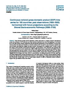
Figure 4. Global distribution of all mesozooplankton biomass Figure 3. Distribution of original sampling depth. Depth interval

0–10 corresponds to zCAT i010; depth interval 0–20 corresponds to zCAT i020, etc. (see Table 4).

using Chauvenet’s criterion; all values being lower than the critical value of the mean +4.6534 × standard deviation. Sampling protocols, handling, preservation and measurement techniques were not considered when removing outliers. These variables are assumed reasonably consistent within COPEPOD, but are most likely not uniform across datasets and projects. Issues related to sampling such as the inherent variability of field populations (Landry et al., 2001), mesh size, type of net, gear avoidance, seasonal/diel vertical migrations, sample handling, e.g., sample splitting, size fractionation and sample analysis, all sources of random sampling error, were considered to have a greater effect than the sampling bias issues found across projects/datasets. 3.2

Biomass description

The mesozooplankton biomass database contains 153 163 data points. Data from a number of stations that have been sampled repeatedly over many years, or programs where measurements have been made on a fine-resolution grid have been included. Therefore, after gridding, we obtained 42 245 data points on the WOA grid (1◦ ×1◦ ×12 months × 33 depths), representing coverage of annually averaged biomass for 20 % of the ocean surface. To limit the overrepresentation of well-sampled locations, we present results of the gridded data. The gridded data were split between regions as follows: 46 % of the data were found in the Pacific Ocean, 16 % in the Atlantic Ocean, 16 % in the Indian Ocean and 14 % in the polar oceans. The tropics, including the equatorial Atlantic, equatorial Pacific, Indian Ocean, which represent 43 % of the ocean surface, accounted for 39 % of the data. In contrast 14 % of the data came from the polar oceans, which represent 5 % of the ocean surface. Only 22 % of the data were found in the Southern Hemisphere (Fig. 4). There is some sampling bias towards the local summer season (Fig. 5e and f), with peak cells found in summer months in both hemispheres. Earth Syst. Sci. Data, 5, 45–55, 2013

data (converted to carbon and a common 333 µm equivalent mesh size). Each point represents a station where mesozooplankton were recorded.

The distribution of biomass values between open water and shelf water was also examined. “Shelf water” was defined as a 1-degree grid cell in an area with a bottom depth of less than 200 m or adjacent to a grid containing land. Globally, the ratio of open vs. shelf water mesozooplankton biomass values was exactly 50 %. However, when Northern and Southern hemispheres are compared, the partitioning between open and shelf water was 47 % to 53 % in the north and 80 % to 20 % in the south; i.e., the Southern Hemisphere data were dominated by open water values. These values reflect the asymmetry in the proportion of samples collected in both hemispheres. Greater shelf water area and greater sampling effort (in terms of samples collected) in the Northern Hemisphere is important to consider when comparing these values. Although open water values seem to dominate the Southern Hemisphere data, biomass values for the region may not necessarily reflect de facto open water environment. Ice cover in the Southern Ocean means that although many samples are collected along the ice edge, the effective coastline, depending upon the season, these are labeled as “open” water by the criteria stated above. 3.3

Global estimates

Global estimates of mesozooplankton biomass were calculated from the gridded data in the top 200 m of the global ocean (see Table 5). Global mesozooplankton biomass had a mean of 5.9 µg C L−1 , a median of 2.7 µg C L−1 and a standard deviation of 10.6 µg C L−1 . Biomass was highest in the Northern Hemisphere, and there were slight decreases from polar oceans (40–90◦ ) to more temperate regions (15–40◦ ) in both hemispheres. Values in the tropics (15◦ N–15◦ S) were intermediate between those at the northern and southern temperate latitudes. The standard deviation within the latitude bands was high so the differences in the mean were not significant. The global total of mesozooplankton carbon biomass in the top 200 m of the ocean was estimated at 0.19 Pg C. This total was www.earth-syst-sci-data.net/5/45/2013/


53

Figure 5. Description of mesozooplankton biomass observations: (a) latitudinal distribution, (b) yearly distribution, (c) latitudinal depth

distribution, (d) depth distribution, (e) monthly distribution in the Northern and (f) Southern hemispheres.

calculated by multiplying the median mesozooplankton biomass value (2.7 µg C L−1 = 2700 µg C m−3 ) × the area of the global ocean (3.56 × 1014 m2 ) × the upper 200 m surface layer (200 m) × 1 × 10−21 µg Pg−1 , which gave a value of 0.19 Pg C. An overview of all 11 PFT groups currently included in the MAREDAT project is given in the Introduction to the MAREDAT ESSD Special Issue (see Buitenhuis et al., 2012). A comparison of all PFT biomasses, e.g., picophytoplankton, diazotrophs, coccolithophores, Phaeocystis, diatoms, picoheterotrophs, microzooplankton, mesozooplankton, pteropods and macrozooplankton, is also presented. It is important to be aware that the majority of the other plankton groups only have a small fraction of the data coverage seen in the mesozooplankton data of this paper. For these groups, the spatial and temporal coverage were limited such that only a basic comparison of “latitudinal ranges” and “annual averages” was possible.


4

Conclusions and recommendations

A coherent map of mesozooplankton global distribution and biomass is presented. Global mesozooplankton biomass was estimated from the median biomass value of 2.7 µg C L−1 (= 0.19 Pg C annual average mesozooplankton biomass in the top 200 m) and a standard deviation of 10.6 µg C L−1 . The global, latitudinal and depth estimates of biomass concentrations will be useful for understanding ocean biogeochemistry, and for evaluating global models that include mesozooplankton. Although less developed versions of the mesozooplankton data have been published before as part of the regular COPEPOD database report series (O’Brien, 2005, 2007, 2010), this is the first time individual mesh categories (mCATs) and depth intervals (zCAT) have been distributed. This is also the first time these data have been collected together as a whole for publication in a journal together with the publication of the associated dataset. The dataset description and methods should act as a guide to those interested in using this dataset. It is important when using a dataset such as this that the associated caveats are understood and should be considered when drawing conclusions based on these data. Earth Syst. Sci. Data, 5, 45–55, 2013

54


(a)

(b)

(c)

(d)

Figure 6. Annual mean mesozooplankton biomass (µg C L−1 ): (a) combined 0–100 m, 0–150, and 0–200 m sampling depth intervals (zCAT

i100 + i150 + i200); (b) 0–100 m sampling depth interval (zCAT i100) (c) 0–150 m sampling depth interval (zCAT i150) and (d) 0–200 m sampling depth interval (zCAT i200). Sampling mesh of ∼ 333 µm in all.

The data compiled for this effort represent over 50 years of sampling effort made by institutions and scientists from around the world. While combined depth, mesh, and method maps such as Figs. 4 and 6a show a nearly global distribution of data, the extent of this coverage disappears quickly when one looks only at data from a specific month. Detailed maps of the monthly data distribution by depth, mesh, and original biomass type are available online at the COPEPOD project website (http://www.st.nmfs.noaa.gov/copepod). Mesozooplankton investigators and policy makers are encouraged to view these maps, as they show clearly that not all regions of the ocean are adequately sampled and the maps may provide guidance for future mesozooplankton monitoring or process studies to fill in these gaps. Communication between biogeochemical modelers, data managers and experimentalists is at an all time high. There is an increasing interest to combine expertise from the modeling and experimental communities to produce and share the data products necessary to parameterize and validate marine ecosystem models. COPEPOD regularly interacts with scientific projects such as MAREMIP and international working groups such as the ICES Working Group on Zooplankton Ecology (WGZE). Through collaboration with the scientists and user community, COPEPOD strives to constantly improve its data content and to ensure data products, such as


the biomass fields in this paper, are available and useful to the scientific community. Acknowledgements. A significant portion of the historical

plankton data content present within COPEPOD is possible through data rescue, digitization, and funding provided by NOAA’s Climate Data Modernization Program (CDMP). We thank Erik Buitenhuis, Meike Vogt and Stéphane Pesant for their support for the duration of this project. Edited by: S. Pesant

References Balvay, P. G.: Equivalence entre quelques parametres estimatifs de l’abondance du zooplankton total, Schweiz. Z. Hydrol., 49, 75– 83, 1987. Beaugrand, G., Brander, K. M., Lindley, J. A., Souissi, S., and Reid, P. C.: Plankton effect on cod recruitment in the North Sea, Nature, 426, 661–664, doi:10.1038/nature02164, 2003. ´ Bode, A., Alvarez-Ossorio, M. T., and Gonzáles, N.: Estimation of mesozooplankton biomass in a coastal upwelling area off NW Spain, J. Plankton Res., 20, 1005–1014, 1998. Bogorov, V. G., Vinograd, M. E, Voronina, N. M., Kanaeva, I. P., and Suetova, I. A.: Distribution of zooplankton biomass within the superficial layer of the world ocean, Dokl. Akad. Nauk SSSR, 182, 1205–1207, 1968.


R. Moriarty and T. D. O’Brien: Distribution of mesozooplankton biomass in the global ocean Buitenhuis, E., Le Quéré, C., Aumont, O., Beaugrand, G., Bunker, A., Hirst, A., Ikeda, T., O’Brien, T., Piontkovski, S., and Straile, D.: Biogeochemical fluxes through mesozooplankton, Global Biogeochem. Cy., 20, GB2003, doi:10.1029/2005gb002511, 2006. Buitenhuis, E. T., Vogt, M., Moriarty, R., Bednarˇsek, N., Doney, S. C., Leblanc, K., Le Quéré, C., Luo, Y.-W., O’Brien, C., O’Brien, T., Peloquin, J., Schiebel, R., and Swan, C.: MAREDAT: towards a World Ocean Atlas of MARine Ecosystem DATa, Earth Syst. Sci. Data Discuss., 5, 1077–1106, doi:10.5194/essdd-51077-2012, 2012. Colton, J. B., Green, J. R., Byron, R. R., and Frisella, J. L.: BONGO net retention rates as effected by towing speed and mesh size, Can. J. Fish. Aquat. Sci., 37, 606–623, doi:10.1139/f80-077, 1980. Cushing, D. H., Humprey, G. H., Banse, K., and Laevastui, T.: Report of the committee on terms and equivalents. Rapp. P.-V. Reun. Cons. Int. Explor. Mer, 144, 15–16, 1958. DeVries, D. R. and Stein, R. A.: Comparison of three zooplankton samplers: a taxon-specific assessment, J. Plankton Res., 13, 53– 59, 1991. Glover, D. M., Jenkins, W. J., and Doney, S. C.: Modeling Methods for Marine Science, Cambridge University Press, Cambridge, 588 pp., 2011. Harris, R. P., Wiebe, P. H., Lenz, J., Skjldal, H. R., and Huntley, M.: ICES Zooplankton Methodology Manual, Academic Press, 684 pp., 2000. Hernroth, L.: Sampling and filtration efficency of 2 commonly used plankton nets – a comparitive study of the Nansen net and the UNESCO WP-2 net, J. Plankton Res., 9, 719–728, doi:10.1093/plankt/9.4.719, 1987. Landry, M. R., Al-Mutairi, H., Selph, K. E., Christensen, S., and Nunnery, S.: Seasonal patterns of mesozooplankton abundance and biomass at Station ALOHA, Deep-Sea Res. Pt. II, 48, 2037– 2061, doi:10.1016/s0967-0645(00)00172-7, 2001. Le Quéré, C., Harrison, S. P., Prentice, I. C., Buitenhuis, E. T., Aumont, O., Bopp, L., Claustre, H., Da Cunha, L. C., Geider, R., Giraud, X., Klaas, C., Kohfeld, K. E., Legendre, L., Manizza, M., Platt, T., Rivkin, R. B., Sathyendranath, S., Uitz, J., Watson, A. J., and Wolf-Gladrow, D.: Ecosystem dynamics based on plankton functional types for global ocean biogeochemistry models, Glob. Change Biol., 11, 2016–2040, 2005.


55

O’Brien, T. D.: COPEPOD: A Global Plankton Database, US Dep. Commerce, NOAA Tech. Memo, 136 pp., 2005. O’Brien, T. D.: COPEPOD: The Global Plankton Database. A review of the 2007 database contents and new quality control methodology, US Dep. Commerce, NOAA Tech. Memo, 28 pp., 2007. O’Brien, T. D.: COPEPOD: The Global Plankton Database. An overview of the 2010 database contents, processing methods, and access interface, US Dep. Commerce, NOAA Tech. Memo NMFS-F/ST-36, 28 pp., 2010. O’Brien, T. D., Conkright, M. E., Boyer, T. P., Stephens, C., Antonov, J. I., Locarnini, R. A., and Garcia, H. E.: World Ocean Atlas 2001, Volume 5: Plankton, NOAA Atlas NESDIS 53, edited by: Levitus, S., US Government Printing Office, Washington DC, 89 pp., 2002. O’Brien, T. D., Wiebe, P. H., and Hay, S.: ICES Zooplankton Status Report 2008/2009, 152 pp., 2011. Reid Jr., J. L.: On Circulation, Phosphate-Phosphorus Content, and Zooplankton Volumes in the Upper Part of the Pacific Ocean, Limnol. Oceanogr., 7, 287–306, 1962. Sieburth, J. M., Smetacek, V., and Lenz, J.: Pelagic Ecosystem Structure: Heterotrophic Compartments of the Plankton and Their Relationship to Plankton Size Fractions, Limnol. Oceanogr., 23, 1256–1263, 1978. Wiebe, P. H.: Functional regression equations for zooplankton displacement volume, wet weight, dry weight, and carbon. A correction, Fish. Bull., 86, 833–835, 1988. Wiebe, P. H., Boyd, S., and Cox, J. L.: Relationships between zooplankton displacement volume, wet weight, dry weight, and carbon, Fish. Bull., 73, 777–786, 1975.
