Wybrzeże Wyspiańskiego 27, 50-370 Wrocław, Poland. bDepartment of Miniinvasive and ..... tions, USA 1980. [14] M. Hagan, M. Menhaj, IEEE Trans. Neural ...
Vol. 118 (2010)
ACTA PHYSICA POLONICA A
No. 6
Optical and Acoustical Methods in Science and Technology
Feed Forward Neural Network for Autofluorescence Imaging Classification Z. Kulasa , E. Bereś-Pawlika and J. Wierzbickib a
Institute of Telecommunications, Teleinformatics and Acoustics, Wrocław University of Technology Wybrzeże Wyspiańskiego 27, 50-370 Wrocław, Poland b Department of Miniinvasive and Proctological Surgery, Wrocław Medical University Borowska 213, 50-556 Wrocław, Poland
The key elements in cancer diagnostics are the early identification and estimation of the tumor growth and its spread in order to determine the area to be operated on. The aim of our study was to develop new methods of analyzing autofluorescence images which will allow us an objective and accurate assessment of the location of a tumor and will also be helpful in determining the advancement of the disease. The proposed classification methods are based on neural network algorithms. An Olympus company endoscopic system was used for an autofluorescence intestine imaging study. The autofluorescence imaging analysis process can be divided into several main stages. The first step is preparation of a training data set. The second one involves selection of feature space, namely the selection of those features which enable distinguishing the pathologically altered areas from the healthy ones. Final stages of the analysis include pathologically changed tissue classification and diagnosis. PACS numbers: 87.57.−s, 87.57.R−, 87.57.nm, 87.19.xu, 87.19.xj
1. Introduction Studies on the use of autofluorescence images for early detection of tumor tissues were presented in the early 1990s. In 1991, Palcić was one of the first to apply fluorescence imaging in the lung imaging fluorescent endoscope (LIFE) system [1]. Lam has demonstrated other successful tests in his works in 1993 and 1998 [2, 3]. The results were confirmed using fluorescence imaging to be five times as effective in lesion detection (such as dysplasia and carcinoma in situ) as using images obtained with conventional white light illumination. In the work [4] the authors have presented one of the first cancerous change early detection system based on a digital analysis of fluorescence images. It was observed that in autofluorescence images lesions were characterized by clearly red color while green blue areas corresponded to healthy tissues. Based on that, the authors proposed a fluorescence image red and green constituent analysis. During that process the system generated a matrix of red to green aspect ratio values. In the cases where the ratio exceeded “1” the area was classified as pathologically changed. In 2005, Kara and associates compared the LIFE system to new generation videoendoscopes, and they drew attention to significant limitations of the LIFE system. The authors argue that it is impossible to define precancerous changes, such as the Barret esophagus neoplasia, using the LIFE system [5, 6]. The reason for that is that the LIFE system only detects green (480–520 nm) and red (> 630 nm) ratio spectra in autofluorescence endo-
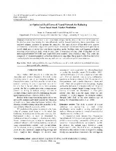
scope images. As a result, various types of inflammation, in which blood flow levels are higher than in healthy tissues, are interpreted by the LIFE system as tumor. It is a result of hemoglobin’s high absorption coefficient for radiation in 500 nm range. The Olympus company has presented a solution to this problem [6]. The source of radiation in the AFI videoendoscope is a 300 W xenon lamp, and two high resolution CCD detectors. What is innovative in the Olympus system is the method of creating autofluorescence images. A set of filters allows a sequential tissue illumination with blue spectrum (395–475 nm) and green spectrum (540–560 nm) radiation every 1/20 s, however, a spectrum filter mounted on the CCD guarantees detection of 490–625 nm spectrum radiation only. The autofluorescence image consists of two basic components: a tissue fluorescence image and an image of green radiation reflected from the tissue. By adding the information about the reflected radiation to an autofluorescence image we are able to distinguish precancerous states (the Barret esophagus neoplasia) and tumors from a local, harmless inflammation [5–9]. Figure 1 shows images of an intestine lesion (polyp). In the case of imaging in white light (1A) separating the lesion from healthy tissue is very difficult, while in the autofluorescence image (1B) the pathologically changed tissue is characterized by clearly different staining, which makes it significantly easier to locate. The aim of our study has been the developing of new methods of endoscopic autofluorescence image analysis
(1189)
1190
Z. Kulas et al.
Fig. 1. Intestine lesion: (A) a standard endoscope image in white light, (B) an autofluorescence image.
green intensity, the third one — proportional to blue intensity, and the fourth table contains the information about the type of tissue a given pixel represents. In this paper, pixel classification into two or three groups has been assumed. When divided into two groups, pixels were classified as pathological area or healthy area. When divided into three groups, the classification involved the creation of an additional “undefined” class, which grouped the objects a decision cannot be unequivocally made about (reflections, shadows). Figure 2 shows the principle of creating a set of training data.
which allow an objective and accurate tumor location assessment, and will help in determining the disease progress degree. The proposed classification methods are based on neural algorithms. In this paper, the objects of classification are autofluorescence images of human intestine. The images have been taken with an Olympus endoscope set at the Wrocław Medical University. 2. Materials and methods The autofluorescence images have been taken during routine colonoscopy and gastroscopy examinations in the Wrocław Medical University. Twenty-five images showing pathological intestinal changes in eleven patients have been chosen from among dozens of recordings. The set of images was divided into two groups: twelve images were used to develop a training set, whereas the remaining thirteen were used to create a testing set. Since in the presented method the classified element is the pixel, over 5000 pixels have been selected from the images chosen for the training set and over 3000 pixels — for the testing set. The training set creation process is presented in Sect. 2.1. Autofluorescence image analysis process can be divided into several stages. The first stage consists of preparing a set of training data. The second stage includes construction of feature space, namely a choice of those features that allow the most effective distinguishing pathologically changed areas from healthy tissues. A classification and diagnosis of tested tissue follow in the last stages of the analysis. 2.1. Training set A training set has been created based on a dozen autofluorescence images depicting precancerous and cancerous tissues. Elements of a training set can be described as follows: U = {hxk , ik i, k = 1, 2, 3 . . . N }. (2.1) Elements of set “U ” can be called examples. Each example consists of full information about the given object’s features vector xk as well as the information on the class number the object is placed in. The training set consists of four tables of equal dimensions. Table elements of the same indices characterize one pixel. The first table contains values proportional to red intensity, the second table — the values proportional to
Fig. 2.
Procedure of creating a training set.
2.2. Feature selection and extraction An assessment of features needed to achieve the task’s usefulness can be made without the need of conducting a full recognition procedure, and can be based just on an analysis of sample distribution that corresponds to different classes in the training set. The further from each other the average values calculated from the samples (pixels) of different classes and the lower standard deviations within these classes, the easier the task of classification will be. If we take under consideration each feature separately, then we deal with a univariate analysis of variance (anova). A discriminant analysis has been proposed in this paper as a method of feature selection, which can easily be reformulated into multivariate analysis of variance (manova) [10–12]. A 6-element feature vector has been generated on the basis of the training set data. The vector consists of values proportional to the intensity of red (R), green (G), blue (B) and component values of the spatial model HSV — hue (H), saturation (S) and value (V). The essence of feature selection by means of discriminant analysis is defining canonical discriminant functions separating our groups. A general form of linear discriminant function has been presented below [12, 13]: Dkj = β0 + β1 x1kj + . . . + βp xpkj , (2.2) where p — number of discriminant variables, N — number of elements, G — number of groups, Dkj — the value of canonical discriminant function for k — the case of the j-th group, k = 1, . . . , N , and j = 1, . . . , G, Xikj — the i
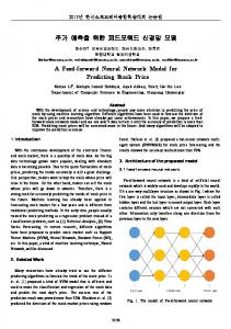
Feed Forward Neural Network . . . value of the discriminant variable for k — the case in j-th group, βi — canonical discriminant function coefficients. Calculating the coefficients of discriminant function is achieved by solving the following equation: (B − λW ) β = 0 (2.3) where B — between group sum of squares, W — within group sum of squares, β — the vector of canonical discriminant function coefficients, λ — eigenvalue. The eigenvalues and eigenvectors are determined based on the above mentioned dependence. Eigenvalues and corresponding vectors are sorted according to the dependence λ1 > λ2 > . . . > λp. In case of the division into three groups only two of the biggest values and their corresponding vectors are considered. Vector elements are canonical discriminant function coefficients. The next step is to standardize coefficients, then calculate structure matrix elements. The standardization of discriminant function coefficients is achieved according to the following formula: s W βp∧ = βp , (2.4) N −g where βp∧ — standardized discriminant function coefficient, βp — non-standardized discriminant function coefficient, W — within group sum of squares, N — number of elements (samples), g — number of groups (p = 3), p — number of discriminatory variables (p = 6). The structure matrix of correlations between predictors and discriminant function, S, is found by multiplying the matrix of within-group correlations among predictors, rik , by a matrix of standardized discriminant function coefficient βp∧ (standardized using pooled within-group standard deviations) [13]: Sp = βp∧ rik , (2.5) where Sp — the structure matrix, βp∧ — standardized discriminant function coefficient, rik — within group correlations. Standardized discriminant function coefficients indicate how strong a given discriminant variable’s impact is on differentiating groups. The higher its value, the bigger the discriminatory impact of the variable. Structure matrix coefficients contribute additional information. They show the strength of interdependence between discriminatory variables and functions. If the coefficient value is close to −1 or 1, it means that all the information about the discriminant function is included in the variable. Structure coefficients are widely used to interpret the discriminant function because they are correlations between variables and discriminant function. By analyzing the coefficients calculated on the basis of picture sets of autofluorescence endoscopy of intestines, we can state that red (R), green (G) color values and value (V) largely contribute to group discrimination. The result of the discriminant analysis presented above is a reduction of the feature space to three dimensions. Figure 3 shows a feature space as well as a distribution of training set data in the 3-class division. Only two dimen-
Fig. 3.
1191
Two-dimensional feature space.
sions of feature space have been shown for a transparent demonstration. 2.3. Classification A feed-forward network with the Levenberg– Marquardt algorithm has been designed for the classification of endoscopic human tissue images. The network consisted of three neurons in the input layer and one neuron in the output layer in the case of dividing images into two classes, and two neurons in the output layer in the case of dividing images into three classes. Additionally, there are two hidden layers. Sigmoid activation function has been applied in the cases of all neurons. The process of classification can be divided into three stages: training the network, testing the network, images classification. The training set consisted of more than 5000 pixels chosen from among 12 images depicting tissues of five different patients. Each example (pixel) in the learning set consisted of information on its characteristics, i.e. R, G, V components as well as the information on whether the pixel represents the “pathological class” or the “healthy class”, or, in the case of a division to three classes, the “pathological class”, the “healthy class”, or the “undefined class”. Applying the Levenberg–Marquardt algorithm makes all the weight of the network update simultaneously, which results in significant reduction of training time even with large numbers of training sets [12, 14]. The testing stage was performed on a set of 3000 pixels, which were prepared on the basis of randomly selected images not involved in the training process. The value of pixels classified incorrectly was 14%. Most of them represented pathological areas. The final stage is the classification process. Two variants of the classification have been assumed in this work, i.e. classification into two groups and classification into three groups. In the case of division into two classes, the network recognizes a given object (pixel) as “pathological” when the output neuron activation level is higher than 0.8. In the case of division to three classes, the network recognizes a given object (pixel) as “pathological”
1192
Z. Kulas et al.
when one output neuron activation level is higher than 0.8 and the other one is lower than 0.2. The resolution of the analyzed image was 384×288 px, which results in over 110 × 103 pixels tested. The time needed for classification of a single frame did not exceed 0.1 s. 3. Results As we have mentioned in Sect. 2.1, pixels were classified into two or three classes. Endoscopic autofluorescence images of pathologically changed intestine in a form of polyp, and classification results are shown in Fig. 4. By analyzing the results we can conclude that the pathological tissue is localized correctly. Unfortunately, in terms of in vivo it is not possible to define a precise boundary of the lesion, hence it is difficult to determine the extent to which an area classified by the program as pathological corresponds to the actual area of the polyp. Major difficulties in the classification of images are frequently occurring reflections and remnants of faeces, which are classified to the “pathological” group. A large part of reflections also is very similar in color to pathological changes, and using filters does not produce intended effects. A solution to this problem is to analyze the sequence of images.
Fig. 5. Autofluorescence image classification results (split into 3 classes): (A), (B) autofluorescence image of intestine with the outlined place of polyp occurrence, (C), (D) the classification results of A and B images, respectively.
Classification into three groups was performed at the next stage. As it was described in Sect. 2.1, areas where it was hard to make a clear decision whether the tissue was pathological or it was healthy were classified into “undefined” group. The assumption was that this group will also include pixels representing shadows as well as those pixels which the filter cuts off as those representing reflections. Figure 5 presents an image sequence taken in 1 s interval. The red area in Fig. 5C and D corresponds to the pixels classified as “pathological” group, the green area — pixels classified as the “healthy” group and the blue color denotes the areas classified as “undefined”. By analyzing the results, we can conclude that despite the very small and invisible lesion, the neural network relatively accurately locates it. Also the “undefined” areas are classified correctly. Unfortunately, some of the pixels that represented small reflections were classified incorrectly as lesion. 4. Conclusions Fig. 4. Autofluorescence image classification results: (A), (B) autofluorescence images of intestine taken in 1 s interval, (C), (D) the classification results of A and B images, respectively.
Figure 4A depicts a large reflection marked with an arrow that was classified as pathological area (Fig. 4C). The reflection is no longer present in the image taken 1 s later (Fig. 4B), however, the area classified as a polyp only slightly changed its shape.
The paper presents a new method of endoscopic gastrointestinal image analysis and classification. The method is based on endoscopic fluorescence image processing and classification. Images derived mainly from the human intestine were used in the studies. By analyzing the results, we can conclude that the proposed method localizes even slightly visible lesions relatively well. The value of pixels classified incorrectly did not exceed 15%. Unfortunately, at this stage of the research we cannot determine the method’s degree of precision in
Feed Forward Neural Network . . . defining the pathologically changed areas, because histological examination of the samples does not define the pathological areas with such a high accuracy. The presented method appears, however, to be useful as a supporting method, the so-called “red flag”, i.e. the doctor performing an examination should pay special attention to the areas indicated by the network as the “pathological” changes. References [1] B. Palcic, S. Lam, J. Hung, C. MacAulay, Chest 99, 742 (1991). [2] S. Lam, C. MacAulay, B. Palcic, Chest 103, 12 (1993). [3] S. Lam, T. Kennedy, M. Unger, Y.E. Miller, D. Gelmont, V. Rusch, B. Gipe, D. Howard, J.C. LeRiche, A. Coldman, A.F. Gazdar, Chest 113, 696 (1998). [4] H. Zeng, A. Weiss, R. Cline, C. MacAulay, Bioimaging 6, 151 (1998). [5] M. Kara, F. Peters, F. Ten Kate, S. van Deventer, F. Fockens, J. Bergman, Gastrointestinal Endoscopy 61, 679 (2005). [6] N. Uedo, H. Iishi, M. Tatsuta, T. Yamada, H. Ogiyama, K. Imanaka, N. Sugimoto, K. Higashino, R. Ishihara, H. Narahara, S. Ishiguro, Gastrointestinal Endoscopy 62, 521 (2005).
1193
[7] W. Curvers, R. Singh, M. Wallace, L. Song, K. Ragunath, H. Wolfsen, F. Ten Kate, P. Fockens, J. Bergman, Gastrointestinal Endoscopy 70, 8 (2009). [8] T. Wang, G. Triadafilopoulos, Gastrointestinal Endoscopy 61, 686 (2005). [9] K. Boparai, F. van den Broek, S. van Eeden, P. Fockens, E. Dekker, Gastrointestinal Endoscopy 70, 947 (2005). [10] A. Mayer-Base, Pattern Recognition for Medical Imaging, Elsevier Academic, Oxford 2004. [11] B.G. Tabachnick, L.S. Fidell, Using Multivariate Statistics, HarperCollins, New York 1996. [12] G. Konieczny, Z. Opilski, T. Pustelny, E. Maciak, Acta Phys. Pol. A 116, 344 (2009). [13] W.L. Kleck, Discriminant Analysis, Sage Publications, USA 1980. [14] M. Hagan, M. Menhaj, IEEE Trans. Neural Networks 5, 989 (1994).