Sparse Allreduce: Efficient Scalable Communication for Power-Law Data
arXiv:1312.3020v1 [cs.DC] 11 Dec 2013
Huasha Zhao Computer Science Division University of California Berkeley, CA 94720
[email protected]
John Canny Computer Science Division University of California Berkeley, CA 94720
[email protected]
Abstract—Many large datasets exhibit power-law statistics: The web graph, social networks, text data, clickthrough data etc. Their adjacency graphs are termed natural graphs, and are known to be difficult to partition. As a consequence most distributed algorithms on these graphs are communicationintensive. Many algorithms on natural graphs involve an Allreduce: a sum or average of partitioned data which is then shared back to the cluster nodes. Examples include PageRank, spectral partitioning, and many machine learning algorithms including regression, factor (topic) models, and clustering. In this paper we describe an efficient and scalable Allreduce primitive for power-law data. We point out scaling problems with existing butterfly and round-robin networks for Sparse Allreduce, and show that a hybrid approach improves on both. Furthermore, we show that Sparse Allreduce stages should be nested instead of cascaded (as in the dense case). And that the optimum throughput Allreduce network should be a butterfly of heterogeneous degree where degree decreases with depth into the network. Finally, a simple replication scheme is introduced to deal with node failures. We present experiments showing significant improvements over existing systems such as PowerGraph and Hadoop. Keywords-Allreduce; butterfly network; fault tolerant; big data;
I. I NTRODUCTION Power-law statistics are the norm for most behavioural datasets, i.e. data generated by people, including the web graph, social networks, text data, clickthrough data etc. By power-law, we mean that the probability distributions of elements in one or both (row and column) dimensions of these matrices follow a function of the form p ∝ d−α
(1)
where d is the degree of that feature (the number of nonzeros in the corresponding row or column). These datasets are large: 40 billion vertices for the web graph, terabytes for social media logs and news archives, and petabytes for large portal logs. Many groups are developing tools to analyze these datasets on clusters [1]–[10]. While cluster approaches have produced useful speedups, they have generally not leveraged single-machine performance either through CPUaccelerated libraries (such as Intel MKL) or using GPUs. Recent work has shown that very large speedups are possible on single nodes [4], [11], and in fact for many common
machine learning problems single node benchmarks now dominate the cluster benchmarks that have appeared in the literature [11]. Its natural to ask if we can further scale single-node performance on clusters of full-accelerated nodes. However, this requires proportional improvements in network primitives if the network is not to be a bottleneck. In this work we are looking to obtain one to two orders of magnitude improvement in the throughput of the Allreduce operation. Allreduce is a rather general primitive that is integral to many distributed graph mining and machine learning algorithms. In an Allreduce, data from each node, which can be represented as a vector vi for node i, is reduced in some fashion (say via a sum) to produce an aggregate X v= vi i=1,...,M
and this aggregate is then shared across all the nodes. In many applications, and in particular when the shared data is large, the vectors vi are sparse. And furthermore, each cluster node may not require all of the sum v but only a sparse subset of it. We call a primitive which provides this capability a Sparse Allreduce. By communicating only those values that are needed by the nodes Sparse Allreduce can achieve orders-of-magnitude speedups over dense approaches. The aim of this paper is to develop a general Sparse Allreduce primitive, and tune it to be as efficient as possible for a given problem. We next show how Sparse Allreduce naturally arises in algorithms such as PageRank, Spectral Clustering, Diameter Estimation, and machine learning algorithms that train on blocks (mini-batches) of data, e.g. those that use Stochastic Gradient Descent(SGD) or Gibbs samplers. A. Applications 1) MiniBatch Machine Learning Algortihms: Recently there has been considerable progress in sub-gradient algorithms [12], [13] which partition a large dataset into minibatches and update the model using sub-gradients, illustrated in Figure 1. Such models achieve many model updates in a single pass over the dataset, and several benchmarks on
large datasets show convergence in a single pass [12]. While sub-gradient algorithms have relatively slow theoretical convergence, in practice they often reach a desired loss level much sooner than other methods for problems including Regression, Support Vector Machines, factor models, and several others. Finally, MCMC algorithms such as Gibbs samplers involve updates to a model on every sample. In practice to reduce communication overhead, the sample updates are batched in very similar fashion to sub-gradient updates [14]. All these algorithms have a common property in terms of the input mini-batch: if the mini-batch involves a subset of features {f1 , . . . , fn }, then a gradient update commonly uses input only from, and only makes updates to, the subset of the model that is projected onto those features. This is easily seen for factor and regression models whose loss function has the form l = f (AX) where X is the input mini-batch, A is a matrix which partly parametrizes the model, and f is in general a non-linear function. The derivative of loss, which defines the SGD update, has the form dl/dA = f 0 (AX)X T from which we can see that the update is a scaled copy of X, and therefore involves the same non-zero features. 2) Iterative Matrix Product: Many graph mining algorithms use repeated matrix-matrix/vector multiplication. Here are some representative examples. PageRank Given the adjacency matrix G of a graph on n vertices with normalized columns (to sum to 1), and P a vector of vertex scores, the PageRank iteration in matrix form is: n−1 1 GP (2) P0 = + n n Diameter Estimation In the HADI [15] algorithm for diameter estimation, the number of neighbours within hop h is encoded in a probabilistic bit-string vector bh . The vector is updated as follows: bh+1 = G ×or bh .
(3)
Again G is the adjacency matrix and operation ×or replaces addition in matrix-vector product is replaced by bitwise OR operation. Spectral Graph Algorithms Spectral methods make use of the eigen-spectrum (some leading set of eigenvalues and eigenvectors) of the graph adjacency matrix. Almost all eigenvalue algorithms use repeated matrix-vector products with the matrix. To present one of these examples in a bit more detail: PageRank provides an ideal motivation for Sparse Allreduce. The dominant step is computing the matrix-vector product
Figure 1: Batch update vs. mini-batch update G P . We assume that edges of adjacency matrix G are distributed across machines with Gi being the share on machine i, and that vertices P are also distributed (usually redundantly) across machines as Pi on machine i. At each iteration, every machine first acquires a sparse input subset Pi corresponding to non-zero columns of its share Gi - for a sparse graph such as a web graph this will be a small fraction of all the columns. It then computes the product Qi = Gi Pi . This product vector is also sparse, and its nonzeros correspond to non-zero rows of Gi . The input vertices Pi and the output vertices Qi are passed to a sparse (sum) Allreduce, and the result loaded into the vectors Pi0 on the next iteration will be the appropriate share of the matrix product GP . Thus a requirement for Sparse Allreduce is that we be able to specify a vertex subset going in, and a different vertex set going out (i.e. whose values are to be computed and returned). B. Summary of Work and Contributions In this paper, we describe Sparse Allreduce, a communication primitive that supports high performance distributed machine learning on sparse data. Our Sparse Allreduce has the following properties: 1) Each network node specifies a sparse vector of output values, and a vector of input indices whose values it wants to obtain from the protocol. 2) Index calculations (configuration) can be separated from value calculations and only computed once for problems where the indices are fixed (e.g. Pagerank iterations). 3) The Sparse Allreduce network is a nested, heterogeneous butterfly. By heterogeneous we mean that the butterfly degree k differs from one layer of the network to another. By nested, we mean that values pass “down” through the network to implement an scatter-reduce, and then back up through the same nodes to implement an allgather. Sparse Allreduce is modular and easy to run, and requires only a mapping from node ids to IP addresses. Our current implementation is in pure Java, making it easy to integrate with Java-based cluster systems like Hadoop, HDFS, Spark, etc.
Figure 2: Allreduce Topologies
The key contributions of this paper are the following: • Sparse Allreduce, a programming primitive that supports efficient parallelization of a wide range of iterative algorithms, including PageRank, diameter estimation, and mini-batch gradient algorithms for Machine Learning, and others. • A number of experiments on large datasets with billions of edges. Experimental results suggest that Sparse Allreduce significantly improves over prior work, by factors of 5-30. • A replication scheme that provides a high-degree of fault-tolerance with modest overhead. We demonstrate that Allreduce with our replication scheme can tolerate √ about M node failures on an M -node network, and that node failures themselves do not slow down the operation. The rest of the paper is organized as follows. Section II reviews existing Allreduce primitives, and highlights their difficulties when applied to large, sparse datasets. Section III introduces Sparse Allreduce, its essential features, and an example network. Section IV and V describe its optimized implementation and fault tolerance respectively. Experimental results are presented in Section VI. We summarize related works in Section VII, and finally Section VIII concludes the paper. II. BACKGROUND : A LLREDUCE ON C LUSTERS Allreduce is a common operation to aggregate local model update in distributed machine learnings. This section reviews the practice of data partition across processors, and popular Allreduce implementations and their limitations. A. AllReduce When data is partitioned across processors, local updates must then be combined by an additive or average reduction, and then redistributed to the hosts. This process is commonly known as Allreduce. Allreduce is commonly implemented with 1) tree structure [16], 2) simple round-robin in fullmesh networks or 3) butterfly topologies [17].
1) Tree Reduce: The tree reduce topology is illustrated in Figure 2(a). The topology uses the lowest overall bandwidth for atomic messages, although it effectively maximizes latency since the delay is set by the slowest path in the tree. It is a reasonable solution for small, dense (fixedsize) messages. A serious limitation for Sparse Allreduce applications is that the entire sum is held and distributed by the bottom half of the network. i.e. the length of the sparse sums is increasing as one goes down the layers of this network, and eventually encompasses the entire sum. Thus the time to compute sums is increasing layer-by-layer and one effectively loses the advantage of parallelism. It is not practical for the problems of interest to us, and we will not discuss it further. 2) Round-Robin Reduce: In round-robin reduce, each processor communicate with all other processors in a circular order, as presented in Figure 2(b). Round-robin reduce achieves asymptotically optimal bandwidth, and optimal latency when packets are sufficiently large to mask setupteardown times. In practice though, this requirement is often not satisfied, and there is no way to tune the network to avoid this problem. Also, the very large (quadratic in M) number of messages make this network more prone to failures due to packet corruption, and sensitive to latency outliers. In our experiment setup of a 64-node Amazon EC2 cluster with 10Gb/s inter-connect, the optimal packets size is 1M10M to mask message sending overhead. As illustrated in Figure 3, for smaller packets, latency dominates the communication process, so the runtime per node will goes up when distributing data to larger clusters. In many problems of interest, and e.g. the Twitter follower’s graph and Yahoo’s web graph, the packet size in each round of communication under a round-robin network is much smaller than optimal. This causes significant inefficiencies. 3) Butterfly Network: In a butterfly network, every node computes some function of the values from its in neighbours (including its own) and outputs to its out neighbours. In the binary case, the neighbours at layer d lie on the edges of hypercube in dimension d with nodes as vertices. The
are PageRank and other matrix power calculations, or largemodel machine learning algorithms such as LDA. To avoid clustering of high-degree vertices with similar indices, we first apply a random hash to the vertex indices (which will effect a random permutation). We then sort and thereafter maintain indices in sorted order - this is part of the data structure creation and we assume it is done before everything else. Figure 3: Scalability of round-robin network of 64 Amazon EC2 nodes cardinality of the neighbour set is called the degree of that layer. Figure 2 demonstrates a 2 × 2 butterfly network and Figure 4 shows a 3 × 2 network. A binary butterfly gives the lowest latency for Allreduce operations when messages have fixed cost. Faults in the basic butterfly network affect the outputs, but on a subset of the nodes. Simple recovery strategies (failover to the sibling just averaged with) can produce complete recovery since every value is computed at two nodes. However, butterfly networks involve higher bandwidth. While these networks are “optimal” in various ways for dense data, they have the problems listed above for sparse data. However, we can hybridize butterfly and round-robin in a way that gives us the good properties of each. Our solution is a d-layer butterfly where each layer has degree k1 , . . . , kd . Communication within each group of ki will use the Allreduce pattern. We adjust ki for each layer to the largest value that avoids saturation (packet sizes below the practical minimum discussed earlier). Because the sum of message lengths decreases as we do down layers of the network, the optimal k-values will also typically decrease. B. Partitions of Power-Law Data As shown in [2], edge partitioning is much more effective for large, power-law datasets than vertex partitioning. The paper [2] describes two edge partitioning schemes, one random and one greedy. Here we will only use random edge partitioning - we feel this is more typically the case for data that is “sitting in the network” although results should be similar for other partitioning schemes. III. S PARSE A LLREDUCE In this section, we describe a typical work flow of distributed machine learning, and introduce Sparse Allreduce. Example usage of Sparse Allreduce is discussed in Section III-B. A. Overview of Sparse AllReduce A typical distributed learning task starts with graph/data partitioning, followed by a sequence of alternating model update and model Allreduce. The “data” may directly represent a graph, or may be a data matrix whose adjacency graph is the structure to be partitioned. Canonical examples
Then the vertex set in a group of k nodes is split into k ranges. Because of the initial index permutation, we are effectively partitioning vertices into k sets randomly, but it is much more efficient to do using the sorted index sets. The partitioning is literally splitting the data into contiguous intervals as show in figure 4, using a linear-time, memorystreaming operation. Each range is sent to one of the neighbours (or to self) in the group. Each node in the layer below receives sparse vectors in one of the sub-ranges and sums them. For performance reasons, we implement the sums of k vectors using a tree direct addition of vectors to a cumulative sum has quadratic complexity. Hashing has very bad memory coherence and is about an order of magnitude slower than coherent addition of sorted indices. For the tree addition, the input vectors form the leaves of the tree. The leaves are grouped together in pairs to form parent nodes, and each parent nodes holds a sum of its children. We continue summing siblings up to a root node. This approach has O(N logk) complexity (N is total length of all vectors) if there were no index collisions. But thanks to the high frequency of such collisions for power-law data, the total lengths of vectors decreases as we go up the tree. This is bounded by a multiplicative factor less than one, so the practical complexity is O(N ) for this stage. In terms of constants, it was about 5x faster overall than a hash table approach. This stage also produces a very helpful compression of the data: i.e. many indices of input vertices collide, and the total length of all vectors across the cluster at the second layer is a fraction of the amount at the first layer. The same process is repeated at the layer below, and continues until we reach the bottom layer of the network. At this point, we will have the sum of all input vectors, and it will be split into narrow and distinct sub-ranges representing R/M where R is the original range of indices, and M is the number of machines. From here on, the algorithm involves only distribution of results (allgather). Each layer passes up the values that were requested by a parent (and whose indices were saved during the configuration step) to that specific parent. The indices of those values are sorted and they lie in distinct ranges, and the parent has only to concatenate them to produce its final output sparse vector.
B. Use Case Examples We provide two methods config and reduce, for the programmers. Configuration involves passing down the outbound indices ( an array of vertex indices to be reduced (outbound) and inbound indices (an array of indices to collect). After configuration, the reduce function is called to obtain the vertex values for the next iteration. The reduce function takes in the vertex values to be reduced (corresponding to outbound vertices) and returns the vertex values for the next update (corresponding to inbound vertices). The following code examples show the usage of our primitive to run the PageRank algorithm and mini-batch update algorithm. PageRank: var out = outbound(G) var in = inbound(G) config(out.indices, in.indices) for(i