Nested Sparse Quantization for Efficient Feature

Nested Sparse Quantization for Efficient Feature Coding Xavier Boix1? , Gemma Roig1? , and Luc Van Gool1,2 1

??

2 Computer Vision Lab, ETH Zurich, Switzerland, KU Leuven, Belgium {boxavier,gemmar,vangool}@vision.ee.ethz.ch

Abstract. Many state-of-the-art methods in object recognition extract features from an image and encode them, followed by a pooling step and classification. Within this processing pipeline, often the encoding step is the bottleneck, for both computational efficiency and performance. We present a novel assignment-based encoding formulation. It allows for the fusion of assignment-based encoding and sparse coding into one formulation. We also use this to design a new, very efficient, encoding. At the heart of our formulation lies a quantization into a set of k-sparse vectors, which we denote as sparse quantization. We design the new encoding as two nested, sparse quantizations. Its efficiency stems from leveraging bitwise representations. In a series of experiments on standard recognition benchmarks, namely Caltech 101, PASCAL VOC 07 and ImageNet, we demonstrate that our method achieves results that are competitive with the state-of-the-art, and requires orders of magnitude less time and memory. Our method is able to encode one million images using 4 CPUs in a single day, while maintaining a good performance.

1

Introduction

Recent research has led to important progress in visual object recognition and classification. Many state-of-the-art object recognition schemes consist of a feedforward architecture, usually divided into feature extraction, feature encoding, spatial pooling, and a classifier [1–3]. Recently, sophisticated encoding and pooling schemes have allowed for learning the different blocks in the pipeline [4, 5]. Feature encoding is one of the most intriguing blocks in a feed-forward architecture. Encoding aims at partitioning the feature descriptor space into informative regions, in order to both generalize towards intra-class variances and discriminate between different categories. Many authors pointed out the significant influence feature encoding has on object recognition performance, and stressed the need for encodings with better generalization properties [6, 7]. The trend has been to introduce refined encodings that certainly generalize better and thus achieve higher levels of performance, but that come at the cost of increasing ? ??

Both first authors contributed equally. We thank Christian Leistner for his support. This work was partially supported by the EU projects FP7-ICT-24314 Interactive Urban Robot (IURO) and FP7-ICT248873 Robotic ADaptation to Humans Adapting to Robots (RADHAR).

2

Xavier Boix, Gemma Roig, and Luc Van Gool

computational complexity. Indeed, feature encoding can be orders of magnitude more demanding than feature extraction and pooling, and it can become the bottleneck of the whole pipeline. For real-time and large scale applications, it is therefore crucial to design efficient feature encoding methods. In the literature, one finds a plethora of feature encoding techniques. One of the most popular is assignment-based coding (AC). AC encodes a feature by assigning it to one or more codebook entries. When combined with average pooling, this corresponds to Bag-of-Words (BoW) [8, 9]. Although simple in principle, it can be computationally demanding, since it requires the calculation of distances between the descriptors and the codebook entries. In particular, its computational cost increases with the size of the codebook and the number of patches [10]. Therefore, several methods were devised to speed up the BoW approach, e.g. [11–13]. Sparse coding has emerged as a powerful alternative to AC, showing better results than AC, especially, when combined with max-pooling [2, 14–16]. In terms of efficiency, however, sparse coding optimizes a convex problem of the size of the codebook length, which makes it comparably slow. Locality-constrained linear encoding (LLC) [17] is an approximation of sparse coding, which speeds it up without a significant loss in performance. The current state-of-the-art in visual classification makes use of super-vector coding [18] and Fisher encoding [19], cf. [3]. Yet, both methods are memory-demanding. Using compression methods, e.g. [19], the Fisher kernel can be made tractable for large-scale applications, but the need for decompression before classification reduces the efficiency again. In this paper, we focus on AC because it is a promising compromise in terms of speed and performance [6]. We introduce a new formulation for AC, and from that, we design a new efficient feature encoding scheme. At the heart of our formulation lies a quantization into a set of k-sparse vectors, which we denote as sparse quantization. It offers a novel viewpoint of AC, which, although algorithmically equivalent to AC, it allows for the unification of AC and sparse coding. In fact, our formulation allows for the design of a new efficient encoding. We coin it ‘Nested Sparse Quantization’ (NSQ), which consists of two feature encodings, in a nested architecture. We first encode the features, and the result is then fed to another feature encoder. Both encoders follow the novel formulation of AC. The first one is instantiated in a way that it is very fast to execute, and since it is build from a hard assignment encoder, it yields a binary vector. The second encoder is fed with this binary vector and thus also becomes very efficient to compute. In the experimental part, we compare NSQ to state-of-the-art methods for object recognition. As we show on various datasets, i.e., Caltech 101, PASCAL VOC 07 and ImageNet, our method demands orders of magnitude less time and memory than those previous approaches, while achieving competitive levels of performance. For instance, it is able to encode one million images in less than 24 hours using one laptop of 4 CPUs and 6GB of disk.

Nested Sparse Quantization for Efficient Feature Coding

3

( 1 1 0 ) ( 0 1 1 )

( 1 0 1 )

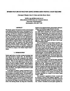
Fig. 1. Representation of B32 (left) and R32 (right) space with the input vector x in green, and the codification error vector (ˆ x − x) in red.

2

Preliminaries

In this section, we introduce the mathematical tools that we use in the rest of the paper, i.e., quantization, sparsity and sparse quantization. All proofs can be found in the appendices. Quantization. Let x ∈ Rq be a vector, and B ∈ Rq×m the so called codebook matrix with m entries bi ∈ Rq , i.e., B = [b1 . . . bm ]. Definition 1. Quantization is a mapping of a vector x into its closest vector of ˆ ? = arg minxˆ ∈{bi } kˆ the codebook {bi |i = 1, . . . , m}, which we denote as x x −xk2 . The purpose of quantization is to reduce the cardinality of the representation space. x has an infinite set of possible values, and when mapped to the codebook, it is restricted to a finite set of possible vectors. In general, the cost of computing a quantization is O(m), where  represents the cost of computing a single distance. In practice, the most common used is the squared Euclidean distance, which is expensive since it implies 2q float operations, and yields a total cost of O(mq). Sparsity. A vector α is k-sparse when it has at most k non-zero entries, i.e., kxk0 ≤ m m m k. Let Rm : k be the space of k-sparse vectors in R , which is Rk = {α ∈ R kαk0 ≤ k}. Sparsity is a highly non-linear model [20]. Observe that the the sum of two k-sparse vectors does not necessarily result in another k-sparse vector, since their non-zero entries might not coincide. Thus, the result is no longer in m Rm k . We also introduce the subset of binary vectors in Rk , which is the set of m m vectors with k ones and (m − k) zeros. Let {0, 1}k = Bk be the space of binary m m k-sparse vectors, Bm : kαk0 = k}, where Bm k = {α ∈ B k is a subset of Rk , m m i.e., Bk ⊂ Rk , and it is composed of a finite amount of elements, in particular,
m its cardinality is |Bm k |= k . Sparse Quantization. We consider the particular case of the quantization when the codebook is the set of k-sparse vectors. Definition 2. Sparse Quantization is a quantization into the codebook B = Rqk .

4

Xavier Boix, Gemma Roig, and Luc Van Gool

The formulation for the sparse quantization of x ∈ Rq is ˆ ? = arg minq kˆ x x − xk2 .

(1)

ˆ ∈Rk x

For brevity, we use the term Sparse Quantization (SQ), but to be more precise, it should be called quantization into the codebook Rqk . Interestingly, sparse quantization can be done in a more efficient way than a quantization into an arbitrary codebook. In the following Proposition, we show that SQ can be achieved with a sorting algorithm, and it does not require the computation of the distances to the codebook entries. The Proposition shows only the case for the codebook Bqk , which is what we use in our approach. The derivation for sparse quantization in the case where the codebook is the set Rqk can be found in the appendix We assume that x ∈ Rq+ , and that x is normalized to 1. In all cases where we use the Proposition this is true. ˆ ? = arg minxˆ ∈Bqk kˆ Proposition 1. Let x x − xk2 be the quantization into Bqk of q ˆ ? by x ∈ R+ , kxk22 = 1. We can obtain x  1 if i ∈ k-Highest(x) ? x ˆi = , (2) 0 otherwise where k-Highest(x) is the set of dimensions indices that indicate which are the k highest values in the vector x. Proposition 1 shows that the sparse quantization can be done with a sorting algorithm of the set {xi }, and selecting the k highest values. It has a computational cost of O(q), in contrast to a general quantization, which has a cost of O(mq), where in practice m  q. In Figure 1, we show an example of sparse quantization in B32 and in R32 . We plot an
input vector x in green, and the quantization error in red. Also, we show all 32 = 3 possible vectors for B32 .

3

A New Formulation of Assignment-based Coding

In this section, we introduce a new framework for Assignment-based Coding (AC), which is based on the principles of sparse quantization. Additionally, we show the relation to Sparse Coding. 3.1

Assignment-based Coding Revisited

We first review AC and its main variants and identify some common terminology in the literature. This will serve as the basis for our new formulation that we introduce in the subsequent section. Let x ∈ Rq+ be the vector of a patch descriptor, which has been normalized, and B ∈ Rq×m the codebook matrix with m entries bi ∈ Rq . AC aims at encoding x by selecting the codebook entries bi with minimum distance to x. Such codebook entries are called the k-Nearest Neighbors (k-NN) of x. k is the number of selected codebook entries, and it is a predefined constant.

Nested Sparse Quantization for Efficient Feature Coding

5

Vector quantization (VQ) is the simplest AC method. It only selects a single codebook entry, which is the closest to x, with the so called 1-NN. It is in fact a quantization, since it maps x into a codebook entry. Let α ∈ Rm be the vector that encodes the assignment. In VQ, αi is set to 1 when it is the element of the codebook that is used to quantize x, and the rest is set to 0. VQ has been extended to the popular hard-assignment (HA), which assigns more than one codebook entry to x, e.g. [12]. In this case, there are 1s placed in the elements of α that correspond to the k-NN codebook entries, i.e.,  1 if i ∈ k-NN(x, B) αi = . (3) 0 otherwise k-NN(x, B) is the set that indicates which k codebook entries are closest to x. According to Definition 1, HA is not a quantization anymore but an assignment, because more than one vector of the codebook is assigned to x. In the case of quantization, x is always represented with only a single codebook vector. In HA, α results in a binary vector with k ones and (m − k) zeros. Thus, the m α’s obtained are k-sparse vectors, which are in Bm k . In particular, α is in Bk m when using HA, and in B1 for VQ. There exists also the soft version of HA, denoted as soft-assignment (SA) [6]1 . In this case, instead of indicating the k-NN with 1s, α contains some notion of the relative distance to the selected codebook entries, and becomes  exp(−βd(x, bi )) if i ∈ k-NN(x, B) αi = . (4) 0 otherwise d(x, y) is a given distance function, β a learned constant, and d(x, bi ) is the distance between x and bi . Thus, SA codifies a patch descriptor x with a km sparse α in Rm k . Note that when β = 0 we recover HA, and α ∈ Bk . AC and other codings are usually the computational bottleneck of the patchbased image classification, cf. [3]. Typically, the cost of coding scales with the number of visual words, the number of patch descriptors and the dimensionality of these descriptors. This can make the coding an order of magnitude slower than the patch description. The reason is mainly because the encoding requires computing the distances between the patch descriptor and all the codebook entries. In the following sections, we introduce a new formulation for AC, that also leads up to a very efficient quantization scheme. 3.2

AC as a Sparse Quantization

We now introduce a new view of AC based on a non-linear mapping of x, which we denote as φ : Rq → Rm . 1

In [6], α is normalized such that kαk22 = 1. In this paper, for the sake of simplicity in the encoding block, we assume it is the pooling stage that normalizes α. Note also that in this paper we refer to SA for what [6] calls Localized SA.

6

Xavier Boix, Gemma Roig, and Luc Van Gool

Definition 3. Let φ(x) be the following mapping: φ(x) =

1 [exp(−βd(x, b1 )) . . . exp(−βd(x, bm ))], Z

(5)

where β is a learned constant and d(a, b) a given distance. Z normalizes the vector, and {b} parametrize the mapping. Observe that in AC, B denotes the codebook matrix, but in our new formulation it is used to parametrize the mapping φ(x). In the following Proposition, we rewrite HA as a sparse quantization of φ(x) (section 2). We show this fact for SA as well as the proof in the appendix. Proposition 2. Let α? ∈ Bm k be the result of Hard Assignment in (3). Then, the same α? can be obtained through the following sparse quantization of φ(x): α? = arg minm ||α − φ(x)||22 . α∈Bk

(6)

Proposition 2 shows that HA is a sparse quantization of φ(x) into the codebook Bm k . HA is formulated as a non-linear transformation φ(x), which uses B, and then the resulting vector is quantized into Bm k . This is in contrast to how HA has been usually interpreted. Previous HA formulations used α in order to indicate to which codebook entries x is assigned. Both formulations obtain the same coding results, and have the same computational complexity. However, in the next subsection we show that Proposition 2 is able to fuse Assignment-based Coding and Sparse Coding into a single formulation. Also, we show that we can use the new formulation to design a very efficient codification. 3.3

A Formulation for Sparse Coding and AC

When considering AC as a sparse quantization, we can analyze its relation to sparse coding. Sparse coding is the following coding scheme [21]: α? = arg minα∈Rm ||Cα−x||22 , where C ∈ Rq×m is the codebook used in sparse coding. k It is usually relaxed in the following way α? = arg minα∈Rm ||Cα−x||22 +λkαk1 , where λkαk1 is the convex sparsity regularization term of α ∈ Rm k , and it can be tuned to enforce different degrees of sparsity. Note that in [15] it was already shown that Sparse Coding can be seen as an extension of VQ; however, their formulation does not extend to AC in general. The general formulation for Sparse Coding and Assignment-based Codings is: α? = arg minm ||Cα − φ(x)||22 , α∈Rk

(7)

where φ(x) represents a mapping from the original q-dimensional vector x to a space with a possibly different dimension, such as m in the earlier definition. We now recover Sparse Coding by just setting φ(x) = x, and we recover AC by setting C to be the identity matrix Im×m .

Nested Sparse Quantization for Efficient Feature Coding

4

7

Nested Sparse Quantization

In this section, we introduce an efficient encoding built upon the new formulation of HA in Proposition 2. It consists of two sparse quantizations placed in a nested architecture, coined nested sparse quantization (NSQ). We define NSQ as the following optimization problem: α = arg minm kα − φ(ˆ x)k2 ,

(8)

ˆ = arg min 0 kˆ where x x − θ(x)k2 ,

(9)

α∈Bk

ˆ ∈Bm x k0

where (8) is the outer sparse quantization and (9) is the inner sparse quantization, respectively. The parameters in the inner quantization are m0 , k 0 and the mapping θ(x), and they are not necessarily the same as in the outer quantizaˆ , as a result of the sparse tion. The inner quantization results in the binary x quantization into Bm . The mapping in the inner quantization θ(x) has the realk 0 ˆ ∈ Bm valued x as input, whereas the outer mapping φ(ˆ x) gets the vector x k0 as input, which is a binary vector. 4.1

Implementation Advantages

Observe that the input to the outer quantization has a finite amount of possible values, because it receives one of the entries of the inner codebook. This allows to use a look up table for the outer quantization, by memorizing the quantization of all entries of the inner codebook. However, in practice, the cardinality of the inner codebook is huge. In NSQ, the outer quantization is a mapping from a


0
m m0 m set of m k0 elements to k possible outputs, where in practice k0  k and they are too high to be memorized in a look up table. Indeed, the advantage of NSQ results from an appropriately chosen nesting of two different quantizations. The inner quantization turns real-valued vectors 0
ˆ , and the non-linear mapping x into one of the m possible binary vectors x k0 should be simple not to overload the system. The outer quantization starts from 0 a vector in the set Bm k0 , which are binary vectors, and can therefore be used to very efficiently deploy a more complex mapping φ(ˆ x). Inner Quantization. For the inner quantization, we use the most efficient and simplistic mapping possible, which is θ(x) = x; that is, the mapping θ(x) does not apply any transformation on x. Thus, the inner quantization in Eq. (9) directly quantizes the input x into the k 0 -sparse codebook for that step, without any previous non-linear mapping. It becomes ˆ = arg minq kˆ x x − xk2 ,

(10)

ˆ ∈Bk0 x

where m0 is equal to q, and k 0 is the only parameter to be set. As stated in Proposition 1, optimizing this problem is equivalent to computing the k 0 -Highest values in {xi }. This implies selecting the k 0 elements of x with the highest values, which has a computational cost of O(q). One could investigate alternatives to θ(x) = x to improve on the classification results, but this would reduce the speed again and is therefore not studied in this paper.

8

Xavier Boix, Gemma Roig, and Luc Van Gool

Algorithm 1: Nested Sparse Quantization ˆ ∈ Bq×m Input: x ∈ Rq+ , B k0 Output: α ˆ ← Set k0 highest values of x to 1 and the rest to 0 x foreach i = {1, . . . , m} do P xj ˆbij ) φi (ˆ x) = qj=1 (ˆ end α ← Set k highest values of φ(ˆ x) to 1 and the rest to 0

Outer Quantization. The outer quantization now gets the binary output of the 0 inner quantization as its input, which is a vector in Bm k0 . The use of binary vectors allows to reduce the complexity by using fast bit-wise comparisons, which most modern CPUs handle with dedicated instructions [22, 23]. Thus, we can afford applying a more sophisticated mapping φ. Recall that the computational cost of such φ(ˆ x) still is O(m), with  the cost of computing the distance. We can reduce ˆ is binary. Thus, the mapping is the same as in the cost  by the very fact that x ˆ x, b ˆ i ). Recall (5) but changing the distance function to a Hamming distance, d(ˆ ˆ that the bi are parameters used in the definition of the non-linear mapping, and do not correspond neither to the codebook vectors of the inner quantization nor to the codebook vectors of the outer quantization. In our case, these are obtained by piping a total of m vectors bi through the inner quantization, thus yielding ˆ i. those b Next, the mapping φ(ˆ x) can be further simplified by dropping the exponential functions, given the equivalence of arg minα with the mapping φ(ˆ x) = 1 ˜ ˆ 1 ) . . . d(ˆ ˜ x, b ˆ m )]. Now, suppose we take d(ˆ ˜ x, b ˆ i ) = Pq (ˆ ˆbij ), [ d(ˆ x , b x j=1 j Z where is the negation of the exclusive OR operator (nxor ). It returns 1 if both elements are equal, and 0 otherwise. This is again very efficient to compute. In Algorithm 1 we depict the implementation of NSQ, which highlights the simplicity and efficiency of the method. 4.2

Discussion

Quantization vs. recognition accuracy At this point the reader may object that NSQ adds an extra quantization step in the feature encoding procedure, and that quantization errors may grow worse, leading to a deteriorated performance. Yet, in recognition, quantization should also allow for sufficient generalization. In the next section, we show that recognition performance is not impaired, but that the speed goes up dramatically. Relation of the Inner Quantization to Binary Embeddings and Hashing. NSQ is not to be confused with Binary Embeddings or Hashing-based methods. The goal of the inner quantization is a first step of feature encoding, and it is not designed to be a fast nearest neighbor extractor nor a fast distance approximator. In fact, in the experiments we show that NSQ is not a good nearest neighbor approximator. Hashing-based methods tackle fast distance computation rather

Nested Sparse Quantization for Efficient Feature Coding

9

than feature encoding, and have been typically used to speed up image retrieval in large-scale databases [24–27]. The binarizations used by these methods range from thresholding linear combinations of input features to solving optimization problems. These have a negligible cost in image retrieval, but not when applied to feature encoding. For example, in Locality Sensing Hashing (LSH) the binary embedding is hn (x) = T (rT x), where r is a projection vector, and T (·) is a threshold function. Hashing uses L different N -dimensional embedding functions h(x) of an image signature x, and thus, the cost of computing h(x) is O(LN q). Hashing is typically used in applications where the cost O(LN q) is negligible compared to the cost of searching the nearest-neighbors, because this search might be among hundreds of thousands of elements. However, in feature encoding, the time of computing h(x) is not negligible anymore, because the nearest neighbor search is only among thousands of elements (the size of the codebook), and in addition, h(x) is computed for each patch. In contrast, the ˆ at a cheap cost O(q). Furtherinner quantization of NSQ obtains the binary x more, the binary embeddings generate each bit independently of the others [26], which is different from NSQ, in which the output bits are dependent since only k of them are 1.

5

Experiments

In this section, we report experiments on different datasets, namely Caltech101 [28], PASCAL VOC 2007 [29] and ImageNet [30]. In none of them we use flipped or blurred images to extend the training set. Caltech 101. It contains 102 different classes with about 50 images per class. We use 3 random splits of 30 images per class for training and the rest for testing, and evaluate it with the average classification accuracy across all classes. We resize the image to have a maximum of 300 pixels per dimension. PASCAL VOC 2007. It consists of a total of 9,963 images with 20 different object classes. Half of the dataset is used for training and the other half for testing. The evaluation is based on the mean average precision (mAP) across all classes. ImageNet. We create a new dataset taking a subset of 1, 065, 687 images of ImageNet. This subset contains images of 909 different classes that do not overlap in the synset. We randomly split this subset into two halfs, one for training and one for testing, maintaining the proportion of images per class. For evaluation, we report the average classification accuracy across all classes. Note that we do not use the protocol of taking the 5 highest scores per image and keeping the best. We resize the image to have a maximum of 300 pixels per dimension. 5.1 Implementation Details Patch Descriptors. We use SIFT [31] extracted from patches on a regular grid, at different scales. In Caltech 101 and ImageNet they are extracted at every 8 pixels and at the scales of 16, 32 and 48 pixels diameter. In VOC07, SIFT is sampled at each 4 pixels and at the scales of 12, 24 and 36 pixels diameter.

10

Xavier Boix, Gemma Roig, and Luc Van Gool

(a)

(b)

(c)

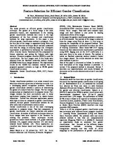
Fig. 2. Influence of the parameter k and the vocabulary size in Caltech 101. (a) Comparison of performance and time between NSQ and HA when varying the size of the codebook. (b) Accuracy and (c) Time when varying the inner and outer quantization parameters.

Feature Encoding. Apart from comparing NSQ and HA, we also report results with LLC [17] and the Super Vector method [18]. We found that for all settings k = 5 is the optimal, except for the combination of HA, max-pooling and linear SVM, which is k = 10. In NSQ, k 0 = 25 for the inner quantization (see discussion in 5.2 for those choices). Codebook Generation. The codebook B is typically built with a learning algorithm either unsupervised [8, 9] or supervised [13]. Recently, Coates and Ng [7] showed that a similar performance can be achieved by randomly picking a set of patches as codebook entries. We compared a codebook obtained using kmeans clustering versus building it taking random patches from the training set. Tallying with the observations in [7], compared to k-means clustering, random selection considerably reduces the training time but does not lower the performance for large codebooks. For the methods that are not AC, like LLC or Super Vector, we learned the vocabularies as specified for each of them. Pooling. We use in all datasets spatial pyramids. In Caltech 101 and ImageNet we divide the image in 4 × 4, 2 × 2 and 1 × 1 regions, yielding 21 different regions, and in VOC07, 3 × 1, 2 × 2 and 1 × 1 regions, yielding 8 regions. We use maxpooling because it has been shown to systematically outperform other types of pooling. In the case of NSQ and HA, the max-pooling results in a binary vector, which is the descriptor of the whole image, which we do not normalize. Classification. For Caltech 101 and VOC07, we use a linear one versus rest SVM classifier for each class with the parameter C of the SVM set to 1000. In Caltech 101, we also report results using the RB-χ2 kernel, exp{−βχ2 }, setting β to the mean of the pairwise distances in the training data. Before computing the χ2 distance, the features are normalized with the `1 -norm. When the image descriptor is binary, the RB-χ2 kernel can be computed efficiently using dedicated CPU instructions [22, 23]. In ImageNet we use as classifier an approximated nearest neighbor that takes a maximum of 400 random examples per class. Computational Evaluation. We use CPUs at 3.07GHz with the SSE4.1 instruction set, that enables fast popcnt instructions for bit strings.

Nested Sparse Quantization for Efficient Feature Coding Method Coding Pool Kernel HA{25,10} Max Linear HA{20,5} Max Linear NSQ HA{20,5} Max RB-χ2 HA{20,5} Sum RB-χ2 HA{10} Max Linear HA{5} Max Linear HA{5} Max RB-χ2 Standard HA{5} Sum RB-χ2 LLC Max Linear SV Max Linear HA [6] Max Linear Other SA [6] Max Linear features LLC [17] Max Linear FK [3] Max Linear

Acc. (%) 74.2 ± .7 73.7 ± .3 72.0 ± .6 71.6 ± .3 74.6 ± .6 74.2 ± .1 73.4 ± .9 72.1 ± .4 76.1 ± .7 76.9 ± .9 73.3 ± .6 74.2 ± .8 73.4 ± − 77.8 ± .6

11

Time per Image 1 CPU (sec) Memory Feature Coding Kernel (Bytes) 0.27 ± .11 0.17 ± .05 − 21K 0.27 ± .11 0.15 ± .05 − 21K 0.27 ± .11 0.15 ± .05 .02 21K 0.27 ± .11 0.17 ± .07 2.10 672K 0.27 ± .11 2.78 ± .9 − 21K 0.27 ± .11 2.75 ± .9 − 21K 0.27 ± .11 2.75 ± .9 .02 21K 0.27 ± .11 2.78 ± .9 2.10 672K 0.27 ± .11 2.95 ± .9 − 672K 0.27 ± .11 1.52 ± .9 − 10752K − − − − − − − − − − − − − − − −

Table 1. Quantitative Results on Caltech 101. The time and memory measurements are for one image. We refer to HA{k0 ,k} for the HA with NSQ, and HA{k} for the standard, in which we indicate the k and k0 parameters of the outer and inner quantizations, respectively.

5.2

Results

Performance Evaluation. In Table 1 we report results in Caltech 101. We show the results for NSQ in combination with different SVM kernels and pooling schemes. We do the same for HA, and we also include a comparison with LLC and Super Vector. We use a codebook of 8, 192 entries for all methods except for Super Vector for which we use 1, 024, since it achieves the compromise between accuracy and efficiency. LLC and Super Vector perform better than the others, as was reported in previous papers. However, their coding consumes much more memory and time than NSQ. The performance of NSQ is only 2.7% less than the best competing method which is Super Vector, but NSQ requires 500 times less memory than Super Vector and is about 10 times faster, and is 20 times faster than other methods that use the same codebook size. In Table 2 we summarize the results in VOC07. We use a codebook size of 16, 258 entries. NSQ obtains a 30 times speed up, while only degrading 2% in performance. In both tables we also provide the state-of-the-art methods in the literature. Even though they obtain better performance than our method, these techniques come at a far higher computational cost, as seen in the previous comparisons. We did not reproduce results of SA because it was already observed by [6] that SA only outperforms HA by less than 1%. Also, note that in VOC07 there is a gap between the performance of LCC reported by [17] and the LCC using our descriptors. According to [3], this can be explained by the fact that [17] extend the training set by blurring and flipping the images, and we do not. Influence of the Parameters. In Figure 2a, we compare time and accuracy when changing the codebook size for NSQ and HA. Up to a certain point, the larger the codebook, the better the accuracy becomes. Interestingly, the computational time for HA explodes when increasing the codebook size, while in NSQ the increase is negligible compared to HA.

53 56 57 53 60

21 22 21 29 34

56 57 60 69 72

72 75 74 79 83

55 56 57 62 64

41 44 43 54 57

48 50 52 49 53

42 43 44 52 63

37 37 42 44 49

65 69 68 67 72

78 78 81 84 85

21 24 24 31 36

45 46 48 45 46

71 74 72 79 83

51 51 52 54 59

Memory

71 74 73 77 81

66 66 70 71 74

Coding Time

41 44 46 51 55

56 56 58 65 72

Feature Time

Sofa Train TV/Monitor

67 67 69 75 79

Average

Horse Motorbike Person Potted Plant Sheep

NSQ HA LLC LLC [17] SV [18]

Bird Boat Bottle Bus Car Cat Chair Cow Dinning Table Dog

Xavier Boix, Gemma Roig, and Luc Van Gool

Aeroplane Bicycle

12

52.87 0.85 0.86 42K 54.54 0.85 21.22 42K 55.56 0.85 23.81 1344K 59.30 − − − 64.00 − − −

Table 2. PASCAL VOC 2007 classification results. The average score provides the per-class average. The time and memory measurements are for one image, using a single CPU.

We analyze the accuracy and time performance of our method when changing the quantization parameters. We use the first split of Caltech 101 to show the results. In Figures 2b and 2c, we compare the accuracy of our method when changing the k parameter for the inner quantization and the outer quantization, and keeping the codebook size at 8, 192. We see a peak of performance: When the inner k is around 20 and 35 and the outer k is around 10 and 16. In the right plot we analyze the time when changing this parameters, also keeping the codebook at size 8, 192. The lower both k are, the less time classification takes. The best compromise between time and performance is using k 0 = 25 for the inner quantization, and k = 10 for the outer. Influence of the Quantization Error. We analyze the impact of having more quantization error due to the inner quantization. We use Caltech 101 to show results using 8, 192 codebook entries. In Figure 3a, we show that the quantization error of the inner quantization does not have a clear relation with the classification accuracy. The accuracy is maximal for k 0 at 20 and 35, and the quantization error has its minimum around 45. Moreover, we show the percentage of equal activated elements of α in NSQ and in HA using the same B, in Figure 3b. Around 90% of the nearest neighbors are different. This shows that NSQ is a new encoding and not an approximate nearest-neighbor. ImageNet in a Laptop in one Day. We introduce a new benchmark to test the efficiency of the encodings. We used ImageNet with restrictions on time and memory, and only let the image encoding algorithms run about 24 hours on a laptop of 4 CPUs. We compared our method with HA with max pooling in which we adjusted the parameters to fulfill the requirements. With NSQ we were able to use a codebook of 2, 048 entries, and in HA only of 256. In Figure 3b the results are summarized. In this benchmark, we outperform HA because in the same amount of time NSQ can use a larger codebook, which is crucial to have good classification performance. The reported results are of the same order of magnitude as reported in [32], though a direct comparison is not possible because we use a different subset of ImageNet. The state-of-the-art for this dataset is

Nested Sparse Quantization for Efficient Feature Coding

Time Dataset Features Coding Total SizeDataset Acc.Top-1

(a)

(b)

13

NSQ

HA

17h 21m 6h 54m 24h 18m 5.4GB 20.01%

17h 21m 7h 9m 24h 30m 700MB 16.6%

(c)

Fig. 3. (a) Quantization error of the inner quantization vs k0 , in Caltech 101. (b) Evaluation of the inner quantization as a nearest neighbor on Caltech 101 changing k and k0 . (c) Quantitative results on ImageNet. To fulfill the time constraints, NSQ uses a codebook of 2, 048 and HA of 256 .

reported by [33], but the computational effort of this method is huge compared to ours.

6

Conclusion

We investigated efficient encoding schemes for object recognition and presented a novel encoding formulation that allows to fuse sparse coding and assignmentbased coding. We proposed a very efficient encoding algorithm called Nested Sparse Quantization (NSQ), which is based on two nested quantizations. The implementation of NSQ is very simple, and can virtually be incorporated everywhere where assignment-based coding schemes are employed, but higher efficiency and more compact representations are demanded, e.g. real-time and large scale recognition problems. This potential was corroborated by our experiments on the Caltech 101, PASCAL VOC 07 and ImageNet benchmarks.

A

Sparse Quantization in Bqk

Recall that we assume that x ∈ Rq+ , and that x is normalized to 1, and recall that the elements of Bqk have norm k. In all cases where we use the Proposition this is true. ˆ ? be x ∈ Rq quantized into Bqk , i.e., x ˆ ? = arg minxˆ ∈Bqk kˆ Proposition 1. Let x x− 2 ? ˆ by setting to 1s the k highest dimensions in x, and 0 xk . We can obtain x otherwise, i.e.,  1 if i ∈ k-Highest(x) x ˆ?i = , (11) 0 otherwise where k-Highest(x) is the set of dimensions indices that indicate which are the k highest values in the vector x.

14

Xavier Boix, Gemma Roig, and Luc Van Gool

P ˆ ∈ Bm Proof. We first rewrite ||ˆ x − x||2 as i (ˆ xi − xi )2 . Since x k has k elements set to 1 and (m − k) set to 0, we can write the above summation as X

(ˆ xi − xi )2 =

i

X

X

(1 − xi )2 +

i:ˆ xi =1

(xi )2 .

(12)

i:ˆ xi =0

We sort in descending order the set of values at each dimension of x, i.e., we sort {xi }, and we use a new indexing in this ordered set. We indicate so by using x0 , and we index it with s instead of i, such that x0(s−1) > x0s . To see when (12) is minimum, note that (x01 )2 > . . . > (x0(s−1) )2 > (x0s )2 > . . .

(13)

(1 − x01 )2 < . . . < (1 − x0(s−1) )2 < (1 − x0s )2 < . . . ,

(14)

where (14) is due to the assumption kxk2 = 1. Therefore, to make both terms in ˆ such that (1 − x0s )2 in (14) are minimum, (12) minimum, we set the k ones in x ˆ such that (x0s )2 in (13) are minimum. Thus, we and we set (m − k) zeros in x set the k ones in the k highest values, and 0 to the other (m − k) values, which is what the Proposition says. t u

B

Sparse Quantization in Rqk

We present the extension of Proposition 1 in the paper to quantize x in the sparse set Rqk . In this case, we assume that x ∈ Rq+ . In all cases where we use the Proposition this is true. ˆ ? be x ∈ Rq quantized into Rqk , i.e., x ˆ ? = arg minxˆ ∈Rqk kˆ Proposition. Let x x− 2 ? ˆ by setting to the xi value the k highest dimensions in x, xk . We can obtain x and 0 otherwise, i.e.,  xi if i ∈ k-Highest(x) ? x ˆi = , (15) 0 otherwise where k-Highest(x) is the set of dimensions indices that indicate which are the k highest values in the vector x. ˆ ? is in the Proof. We can proceed as in Pthe proof 2of Proposition 1, but instead, x m set Rk . The minimum of i (ˆ xi − xi ) is achieved when i : x ˆi = 0 selects the lowest xi . Thus, X X X X (ˆ xi − xi )2 = (xi − xi )2 + (xi )2 = (xi )2 . (16) i

i:ˆ xi 6=0

i:ˆ xi =0

i:ˆ xi =0

This is the same as selecting the k highest elements of x, and setting x ˆ i = xi , and 0 otherwise. t u

Nested Sparse Quantization for Efficient Feature Coding

C

15

HA as a Sparse Quantization

We present the proof for the Proposition of Hard Assignment as Sparse Quantization of the mapping φ(x). Proposition 2. Let α? ∈ Bm k be the result of Hard Assignment in (3). Then, the same α? can be obtained through the following sparse quantization of φ(x): α? = arg minm ||α − φ(x)||22 α∈Bk

Proof (Sketch). We apply Proposition 1 in (17), and we obtain that  1 if i ∈ k-Highest(φ(x)) ? αi = . 0 otherwise

(17)

(18)

Finally, note that k-Highest(φ(x)) is equivalent to k-NN(x, B), and we recover the HA formulation. t u

D

SA as a Sparse Quantization

We now rewrite SA as a sparse quantization of φ(x) in Rqk . Soft-Assignment [6] is defined such that  exp(−βd(x, bi )) if i ∈ k-NN(x, B) ? αi = , (19) 0 otherwise where k-NN(x, B) is the set that indicates which k codebook entries are closer to x, β is a learned constant and d(a, b) is a given distance. Proposition. Let α? ∈ Rm k be the result of Soft-assignment [6] of x to the codebook B, as in (19). Then, α? can also be obtained through the following sparse quantization of φ(x): α? = arg minm ||α − φ(x)||2 α∈Rk

Proof (Sketch). We apply (15) in (20), and we obtain that  φi (x) if i ∈ k-Highest(φ(x)) αi? = . 0 otherwise

(20)

(21)

Finally, note that k-Highest(φ(x)) is equivalent to k-NN(x, B), and together with Definition 3 of the paper, we recover the SA formulation of (19). t u This shows that SA can also be seen as a quantization. That is, SA is equivalent m to quantizing φ(x) into Rm k by selecting the vector in Rk closer to φ(x). In [6], 2 the resultant α is normalized such that kαk = 1. In this paper, for the sake of simplicity in the codication, we consider that is the pooling stage who normalizes α. In the right hand-side of Figure 2 of the paper we show an example of SA in R32 .

16

Xavier Boix, Gemma Roig, and Luc Van Gool

References 1. Boiman, O., Shechtman, E., Irani, M.: In defense of nearest-neighbor based image classification. In: CVPR. (2008) 2. Boureau, Y., Bach, F., LeCun, Y., Ponce, J.: Learning mid-level features for recognition. In: CVPR. (2010) 3. Chatfield, K., Lempitsky, V., Vedaldi, A., Zisserman, A.: The devil is in the details: An evaluation of recent feature encoding methods. In: BMVC. (2011) 4. Zeiler, M.D., Taylor, G.W., Fergus, R.: Adaptive deconvolutional networks for mid and high level feature learning. In: ICCV. (2011) 5. Yu, K., Lin, Y., Lafferty, J.: Learning image representations from pixel level via hierarchical sparse coding. In: CVPR. (2011) 6. Liu, L., Wang, L., Liu, X.: In defence of soft-assignment coding. In: ICCV. (2011) 7. Coates, A., Ng, A.: The importance of encoding versus training with sparse coding and vector quantization. In: ICML. (2011) 8. Csurka, G., Dance, C., Fan, L., Willamowski, J., Bray, C.: Visual categorization with bags of keypoints. In: ECCV. (2004) 9. Sivic, J., Zisserman, A.: Video google: A text retrieval approach to object matching in videos. In: ICCV. (2003) 10. Nowak, E., Jurie, F., Triggs, B.: Sampling strategies for bag-of-features image categorization. In: ECCV. (2006) 11. Nister, D., Stewenius, H.: Scalable recognition with a vocabulary tree. In: CVPR. (2006) 12. Philbin, J., Chum, O., Isard, M., Sivic, J., Zisserman, A.: Lost in quantization: Improving particular object retrieval in large scale image databases. In: CVPR. (2008) 13. Moosmann, F., Jurie, F., Triggs, B.: Fast discriminative visual codebooks using randomized clustering forests. In: NIPS. (2007) 14. Boureau, Y., Ponce, J., LeCun, Y.: A theoretical analysis of feature pooling in vision algorithms. In: NIPS. (2010) 15. Yang, J., Yu, K., Gong, Y., Huang, T.: Linear spatial pyramid matching using sparse coding for image classification. In: CVPR. (2009) 16. Benoit, L., Mairal, J., Bach, F., Ponce, J.: Sparse image representation with epitomes. In: CVPR. (2011) 17. Wang, J., Yang, J., Yu, K., Lv, F., Huang, T., Gong, Y.: Locality-constrained linear coding for image classification. In: CVPR. (2010) 18. Zhou, X., Yu, K., Zhang, T., Huang, T.: Image classification using super vector coding of local image descriptors. In: ECCV. (2010) 19. Perronin, F., Sanchez, J., Mensink, T.: Improving the fisher kernel for large-scale image classification. In: ECCV. (2010) 20. DeVore, R.: Nonlinear approximation. Acta Numerica (1998) 21. Olshausen, B., Field, D.J.: Sparse coding with an overcomplete basis set: A strategy employed by v1? Vis. Res. (1997) 22. Shakhnarovich, G.: Learning Task-Specic Similarity. PhD thesis, Massachusetts Institute of Technology (2005) 23. Calonder, M., Lepetit, V., Strecha, C., Fua, P.: Brief: Binary robust independent elementary features. In: ECCV. (2010) 24. Indyk, P., Motwani, R.: Approximate nearest neighbors: towards removing the curse of dimensionality. In: STOC. (1998) 25. Weiss, Y., Torralba, A., Fergus, R.: Spectral hashing. In: NIPS. (2008)

Nested Sparse Quantization for Efficient Feature Coding

17

26. Gordo, A., Perronnin, F.: Asymmetric distances for binary embeddings. In: CVPR. (2011) 27. Herv´e J´egou, Matthijs Douze, C.S.: Product quantization for nearest neighbor search. PAMI (2011) 28. Fei-Fei, L., Fergus, R., Perona, P.: One-shot learning of object categories. PAMI (2006) 29. Everingham, M., Van Gool, L., Williams, C.K.I., Winn, J., Zisserman, A.: The PASCAL Visual Object Classes Challenge 2007 (VOC2007) Results 30. Deng, J., Dong, W., Socher, R., Li, L.J., Li, K., Fei-Fei, L.: ImageNet: A LargeScale Hierarchical Image Database. In: CVPR09. (2009) 31. Lowe, D.: Distinctive image features from scale-invariant keypoints. IJCV (2004) 32. Deng, J., Berg, A.C., Li, K., Fei-Fei, L.: What does classifying more than 10,000 image categories tell us? In: ECCV. (2010) 33. Lin, Y., Lv, F., Zhu, S., Yang, M., Cour, T., Yu, K.: Large-scale image classification: fast feature extraction and svm training. In: CVPR. (2011)