ORIGINAL ARTICLE
Filling the Gaps: Spatial Interpolation of Residential Survey Data in the Estimation of Neighborhood Characteristics Amy H. Auchincloss,* Ana V. Diez Roux,* Daniel G. Brown,† Trivellore E. Raghunathan,‡ and Christine A. Erdmann* Abstract: The measurement of area-level attributes remains a major challenge in studies of neighborhood health effects. Even when neighborhood survey data are collected, they necessarily have incomplete spatial coverage. We investigated whether interpolation of neighborhood survey data was aided by information on spatial dependencies and supplementary data. Neighborhood “availability of healthy foods” was measured in a population-based survey of 5186 persons in Baltimore, New York, and Forsyth County (North Carolina). The following supplementary data were compiled from Census 2000 and InfoUSA, Inc.: distance to supermarkets, density of supermarkets and fruit and vegetable stores, housing density, distance to a high-income area, and percent of households that do not own a vehicle. We compared 4 interpolation models (ordinary least squares, residual kriging, spatial error regression, and thin-plate splines) using error statistics and Pearson correlation coefficients (r) from repeated replications of cross-validations. There was positive spatial autocorrelation in neighborhood availability of healthy foods (by site, Moran coefficient range ⫽ 0.10 – 0.28; all P ⬍ 0.0001). Prediction performances were generally similar for the evaluated models (r ⬇ 0.35 for Baltimore and Forsyth; r ⬇ 0.54 for New York). Supplementary data accounted for much of the spatial autocorrelation and, thus, spatial modeling was only advantageous when spatial correlation was at least moderate. A variety of interpolation techniques will likely need to be utilized in order to increase the data available for examining health effects of residential environments. The most appropriate method will vary depending on the construct
Submitted 15 September 2006; accepted 19 February 2007. From the *Department of Epidemiology, School of Public Health; †School of Natural Resources and Environment; and ‡Department of Biostatistics, School of Public Health, University of Michigan, Ann Arbor, Michigan. Supported by the National Heart, Lung, and Blood Institute R01 HL071759 and the National Institute on Child and Human Development 1R24 HD047861. AHA designed the study, conducted all analyses, and drafted the manuscript. ADR provided survey data used in this study, assisted with planning analyses, and critically edited the manuscript. DGB assisted in designing the study, interpreted findings, and critically reviewed the manuscript. TER assisted with formulating statistical analyses and critically reviewed the manuscript. CAE critically reviewed the manuscript. Correspondence: Amy H. Auchincloss, Department of Epidemiology, School of Public Health, University of Michigan, 1214 South University 2nd floor, Ann Arbor, MI 48104. E-mail:
[email protected]. Copyright © 2007 by Lippincott Williams & Wilkins ISSN: 1044-3983/07/1804-0469 DOI: 10.1097/EDE.0b013e3180646320
Epidemiology • Volume 18, Number 4, July 2007
of interest, availability of relevant supplementary data, and types of observed spatial patterns. (Epidemiology 2007;18: 469 – 478)
G
rowing evidence supports the concept that residential neighborhoods play a role in determining individual behaviors that are linked to health outcomes.1–3 However, there is a scarcity of relevant data for characterizing neighborhoods that continues to challenge researchers. One option for obtaining information on neighborhoods is to conduct surveys of residents who can provide information about their residential environment. However, survey data necessarily have incomplete spatial coverage. Routinely collected data such as census data have complete coverage but may not provide direct measures of the construct of interest. Geologists and other natural scientists have used geostatistical methods to interpolate when there is incomplete spatial sampling4 –7 and have used supplementary data at colocated sites to try to improve predictions at the unsampled locations.8,9 While spatial modeling in itself may predict reasonably well, supplementary data that are well-correlated with the primary data should improve prediction over and above models of spatial variation alone. We investigated the utility of spatial interpolation methods to obtain estimates of neighborhood characteristics (specifically “availability of healthy foods”) at unsampled locations. We also explored the extent to which spatially complete (and colocated) supplementary data improved the prediction of neighborhood characteristics at unsampled locations. Our hypotheses were: there is positive spatial autocorrelation in the availability of healthy foods in our study sites; supplementary data yield a superior prediction compared with models that do not use these data; and use of spatial information (ie, spatial correlation or conditioning on location) will improve prediction over models that do not incorporate spatial information. Finally, we compared prediction results to determine the best model for predicting the neighborhood characteristic (availability of healthy foods) for our 3 study sites.
METHODS Data Sources of data used in these analyses are listed in Table 1. The primary survey data came from the Community
469
Epidemiology • Volume 18, Number 4, July 2007
Auchincloss et al
TABLE 1. Distribution of “Availability of Healthy Foods” Scale and Area Characteristics by Study Site Using Data From the Community Survey (n ⫽ 5186), 2004, InfoUSA 2003, and Census 2000 Baltimore
Original Data Source
Study area dimensions: No. of Community Survey respondents: Type of Data Computed Variables
Forsyth Co.
New York
36 km ⫻ 20 km 42 km ⫻ 32 km 28 km ⫻ 11 km 1587 1493 2106 Distribution of Variables for Community Survey Respondents Median (25th–75th percentile)
Community Survey, 2004 InfoUSA, Inc., 2003
Survey scale
“Availability of healthy foods”*
3.52 (2.56–4.06)
3.40 (2.43–4.03)
3.76 (3.03–4.24)
Food stores
0.95 (0.58–1.46) 2 (1–4)
1.68 (1.04–2.51) 0 (0–1)
0.30 (0.18–0.48) 18 (12–25)
Census, 2000
Other area characteristics
Distance to supermarkets (km)† Number of supermarkets and fruit/ vegetable stores combined within a 1.6 km‡ Housing density within 1.6 km§ Distance to high-income area (km)¶ Average percent of households within a 1.6 km area that do not own a vehicle
9200 (5000–14,300) 1.69 (0.59–3.35) 20% (8%–35%)
1800 (1000–2900) 2.14 (0.41–5.84) 5% (3%–8%)
72,300 (57,500–94,800) 0.32 (0–1.1) 73% (69%–76%)
*“Availability of healthy foods” scale was based on the mean for: (1) “A large selection of fresh fruits and vegetables is available in my neighborhood;” (2) “The fresh fruits and vegetables in my neighborhood are of high quality;” and (3) “A large selection of low-fat foods is available in my neighborhood.” Survey estimates were weighted to account for differential probabilities of selection into the sample; estimates were also adjusted for age and sex. † Euclidean distance from the survey respondent’s residence to the nearest supermarket. There were 85 supermarkets in Baltimore, 38 in Forsyth Co., and 87 in New York. ‡ There were 116 supermarkets plus fruit/vegetable stores in Baltimore, 43 in Forsyth, and 186 in New York. § Census block group housing units were apportioned over the area of the block group and then summed across a 1.6-km buffer. ¶ Euclidean distance to a high-income area defined as a block group in the top 10th percentile of US per capita incomes ($33,000).
Survey, a population based random-digit-dialing telephone survey.10 Data were collected in 2004 from 5988 residents in Baltimore City/County, Maryland; Forsyth County, North Carolina; Northern Manhattan and Bronx, New York. While the Forsyth site was the most rural of the 3 sites, it did include the cities of Winston-Salem and Kernersville. The Community Survey collected information on a number of neighborhood-level domains potentially related to cardiovascular disease, including neighborhood “availability of healthy foods” which was a scale derived from the mean participant score on 3 items (Table 1 footnote). Participants were asked to report on the area within 1 mile (1.6 km) from their home and to choose from Likert-responses that ranged from 1 ⫽ strongly disagree (unfavorable) to 5 ⫽ strongly agree (favorable). Both scale internal consistency and test-retest reliability (2 weeks postsurvey) were acceptably high (Cronbach’s alpha ⫽ 0.78; test-retest ⫽ 0.69).10 Survey estimates were weighted to account for the differential probabilities of selection into the sample. Survey estimates also were adjusted for age and sex to account for reporting differences by age or sex. We used the adjusted healthy food scale in all analyses. Among 5988 participants, 325 were excluded because of missing data, and 477 survey scores for respondents living within 29 m of each other were averaged together (because geostatistical procedures require that distances between observations not approximate zero and because raster cell size was 20 m2), thus, leaving 5186 observations for these analyses. Potential predictors of availability of healthy foods included 2003 food store data extracted from InfoUSA, Inc.,11 and 2000 US Census block group data.12 We selected supplementary data a priori based on theory and empirical
470
relations found in prior work. Food stores were identified based on Standard Industrial Classifications in the InfoUSA data.13 Because supermarket proximity has been related to availability of healthy foods,14,15 supermarket location was used in 2 measures: distance to supermarkets and density of supermarkets. Supermarket density also included retail fruit and vegetable stores because these stores also may contribute to the availability of healthy foods. Census-derived data included housing density, percent of households without a vehicle, and distance to a high income area. We included housing density because it may be positively related to availability of food resources. Vehicle data were included because automobile transport may influence perceived availability of healthy foods.16,17 In addition, both vehicle and housing variables capture city and suburban differences in food availability. High income areas were included because they have been associated with greater availability of healthy foods.18 Estimated grids (using a 20 m2 cell size) were computed from the supplementary data, and grid values were extracted for survey respondents’ residential addresses (latitude, longitude).
Statistical Analysis Analyses were done separately for each study site. Models fit to the healthy food scale at surveyed points were used to predict availability of healthy foods at unobserved locations. We used model-fit statistics and estimates of regression coefficients from ordinary least squares to evaluate the importance of supplementary data (also referred to as “covariate” information) in predicting food availability. Semivariograms (described below) and the Moran coefficient19 –21 were used to describe/quantify spatial auto© 2007 Lippincott Williams & Wilkins
Epidemiology • Volume 18, Number 4, July 2007
Spatial Interpolation of Residential Survey Data
correlation among original survey values and among ordinary least squares residuals. Four types of prediction models were fit in order to assess the impact of different ways of modeling the spatial correlation in the data. Each of the 4 models is briefly described below. Models were fit both with and without covariates to contrast prediction performance when supplementary data were added to spatial information.
Model 1 Parametric Mean and Independent Covariance—Fitted With Ordinary Least Squares We selected ordinary least squares, a widely-used method for aspatial prediction, to assess whether covariate information applied in a global aspatial regression model would be sufficient for prediction. Ordinary least squares was the benchmark to which all other models were compared. Using k covariates (X) at locations not sampled (j), unbiased predicted values for unobserved Y were derived by applying mean Y (intercept, ) plus the regression coefficients () obtained when Y was observed. This is illustrated by:
investigate the most appropriate functional form for these data. To derive a smoothed plot, semivariogram values were binned into intervals (lag-size). To ensure that bins had sufficient data, in each bin ⱖ80% of surveyed participants were paired with at least one other participant. Model parameters for spatial continuity were derived by noting the distance at which samples ceased to be positively correlated (the spatial “range”), the maximum covariation between samples (the “sill”), and semivariogram values at the origin (measurement error/microscale covariation, the “nugget”). The model parametric functional form was selected by visually comparing plots fit using spherical, exponential, and Gaussian functions, and then subsequently fitting and refitting at least 3 candidate spatial parameterizations with the goal of minimizing root mean square error. Results are presented for the best fitting model. Because patterns in covariation may vary by direction, anisotropic variograms also were examined. All models were specified with a nugget parameter. The spatial dependence function for ordinary kriging of residuals can be written as:
k
Yˆj ⫽ ˆ ⫹
兺 ˆ X . k
(1)
jk
k⫽1
Model 2 Spatial Covariance—Fitted With Residual Kriging If “availability of healthy foods” is spatially autocorrelated and covariate information does not fully account for that pattern, then using spatial dependencies in the data could benefit prediction. We applied residual kriging to assess whether global aspatial prediction by ordinary least squares would be improved by local spatial information remaining in the residuals. Kriging is a spatial interpolation method widely used by geologists and natural scientists, though relatively infrequently used in epidemiology.22–24 Kriging utilizes a weighted linear combination of the available data to obtain an exact best linear unbiased predictor.4,7 In model 2, predictions for unsampled locations were obtained by adding together predicted values from ordinary least squares regression and predicted values obtained from ordinary kriging of the regression residuals, illustrated in simple form as: n
Yˆj ⫹ ˆ j where ˆ j ⫽
兺w . i i
(2)
i⫽1
ˆ j is the ordinary least squares residual predicted at unsampled location j; n is the number of sampled (nearby) residuals (i) that participate in the estimation; and wi are their weights with the constraint that all weights sum to 1 (so as to be unbiased and minimize the mean square prediction error). In order to obtain the weights, ordinary kriging requires prespecification of both a functional form for spatial dependence and the associated parameters for spatial continuity. We used semivariograms (regular and robust),5,25 which plot the covariation of the healthy foods scale as a function of geographic distance between sampled pairs, to © 2007 Lippincott Williams & Wilkins
Cov{i ,j } ⫽ 2 f 共dij , 兲,
(3)
where 2 is the sill, f() is the parametric functional form that uses the distance (d) between locations i and j and the spatial range (). Ordinary kriging of the sampled values also was used to derive predicted values without covariate information.
Model 3 Spatial Covariance—Fitted as Spatial Error Spatial error regression was used to assess whether global ordinary least squares prediction would be improved by simultaneously modeling spatial dependence while estimating the relationship between observed Y and covariates. Predicted values were derived from the following equation: k
Yi ⫽ ⫹
兺 X k
ik
⫹ i , where Cov{i,j} ⫽ 2f (dij,).
k⫽1
(4) The spatial dependency function (illustrated in equation 4 as the covariance between locations i and j) and its parameters were the same as those determined for model 2, with 2 principal differences between model 3 and model 2. First, model 2 used a 2-step approach: supplementary data were fit in ordinary least squares; spatial interpolation (kriging) was performed on residuals; and resultant predicted values were subsequently added to ordinary least squares predictions. In model 3, spatial interpolation was performed by simultaneously modeling supplementary data and the spatial autocorrelation. In model 3, the spatial dependency function was applied such that predicted values were spatially weighted averages of both observed Y and the observed relationship between Y and covariates (X). Second, restricted/residual maximum likelihood was used to estimate simultaneously the mean ( and ) and covariance parameters.26,27
471
Epidemiology • Volume 18, Number 4, July 2007
Auchincloss et al
Model 4 Nonparametric Mean—Fitted With Spline Spline regression was selected to assess whether global ordinary least squares prediction would be improved by modeling spatial trend using a deterministic distribution-free approach. In contrast to the 2 previous models, the functional relationship between spatial location (geographic coordinates: z1, z2) and the dependent variable Y was assumed to be unknown and so was modeled using thin-plate splines (without tension).28 Penalized least squares was used to fit the model while simultaneously using generalized cross-validation to select the optimal smoothing (degrees of freedom or “knots”) for the splines.26 Predicted values for this model were obtained using: k
兺 ˆ X
Yˆj ⫽ f共z1j ,z2j 兲 ⫹
k
jk
(5)
k ⫽ 1
Model Diagnostics Multivariable regression variance inflation factors were examined to determine if multicollinearity barred interpretation of coefficients derived using ordinary least squares. An inflation factor of 10 was used to define high multicollinearity.29 We also examined whether the mean and variance were approximately constant throughout each region (first-order spatial stationarity).4 This was broadly investigated by first examining maps and scatter plots of residuals against predicted values. Second, model 1 fit statistics (Akaike information criterion) were examined before and after adding x, y coordinates (polynomial trend analyses using first and second-order polynomials and interactions30). Finally, maps of predicted values were compared with maps of the original data to assess if predicted values appeared to be reasonable.
Validation The predictive performance of the models was evaluated using repeated replications of cross-validations.31,32 One-third of the observed data at each site was selected randomly and set aside as the validation data. Models fitted to the remaining two-thirds of the data were used to predict values for the validation data and then predicted values were compared with the validation data using root mean square error (RMSE), mean error (ME), mean absolute error (MAE), and Pearson linear correlation coefficients.4,8
RMSE ⫽
ME ⫽
MAE ⫽
472
冑
1 n
1 n
兺(y ⫺yˆ ) ; 2
i
i
i⫽1
n
兺y ⫺yˆ ; i
i
i⫽1
1 n
n
n
兺y ⫺yˆ i
i⫽1
i
(6)
To examine how much variability remained in the predicted values, we also examined standard deviations of the predicted values relative to the standard deviation of the original survey scale. Cross-validations were repeated 100 times to obtain the distribution of the sampling error. All analyses were conducted using SAS v. 8.0 (SAS Institute, Cary, NC) except for the Moran coefficient, which was estimated using S⫹ SpatialStats v. 1.5 Supplement (MathSoft, Needham, MA).
RESULTS The mean values of the “availability of healthy foods” scale were highest in New York City and lowest in Forsyth County (Table 1). Other area characteristics differed considerably across the sites. The Forsyth site had the lowest population density, relatively poor proximity to food stores, and a relatively high level of vehicle ownership. The New York site was the most urban with relatively high proximity to food stores and high percent of households that did not own a vehicle. Area characteristics in Baltimore were intermediate to these two. There was high bivariate collinearity between 2 covariates in Baltimore and in New York, although multivariable collinearity was only moderate for those same variables/sites 关housing unit density and vehicle ownership in Baltimore (bivariate Pearson r ⫽ 0.90, regression inflation factor ⱕ7), and housing density and food store density in New York (bivariate Pearson r ⫽ 0.80 and regression inflation factor ⱕ5)兴. Multicollinearity was low for all other variables/sites (inflation factor ⬍3.0), thus, broad interpretation of the ordinary least squares beta coefficients was possible. In the ordinary least squares models, the relationship between supplementary data and the availability of healthy foods scale was generally in the expected direction at all sites (Table 2): ie, negative for distances to supermarkets, distance to a high-income area, and percent of households that did not own a vehicle; and positive for density of food stores (except for NY) and high housing density. Covariates provided the strongest predictive power in New York (adjusted R2: NY ⫽ 25%; Baltimore ⫽ 11%; Forsyth ⫽ 12%). New York variables with the strongest predictive capacity were distance to a high-income area (partial R2 ⫽ 0.22, not shown); in Baltimore the strongest variables were percent of households that did not own a vehicle and distance to a supermarket (partial R2 0.05 and 0.03, respectively); and in Forsyth County the strongest variable was distance to a supermarket (partial R2 0.10). Diagnostics suggested that there was nonstationarity in New York (not shown): directional semivariograms of the original survey scale revealed periodicity and zonal anisotropy and there was evidence of a trend. Covariate information reduced nonstationarity; therefore, directional spatial dependence was modeled only in New York when covariates were absent in models 2 and 3. In contrast, the Baltimore and Forsyth sites generally had acceptable stationarity. In general, model variograms fit the data reasonably well (Fig. 1) and maps of predicted values and observed residuals appeared reasonable for all the study sites. © 2007 Lippincott Williams & Wilkins
© 2007 Lippincott Williams & Wilkins ⱕ25% ⬎25%
ⱕ1.5km ⬎1.5km
Linear Spline Cut-Points*
⫺1.5173 (0.5168) 0.0034 ⫺3.0394 (0.4280) 0.0000
⫺0.0662 (0.0312) ⫺0.0089 (0.0137) ⫺1.4362 (0.5273)
⫺0.0635 (0.0159) 0.0001
0.0342 0.5153 0.0065
0.7579
⫺0.1238 (0.4016)
0.0000
0.0680 (0.1100) 0.5364
0.1883 (0.0277)
3.7844 (0.1150)
P
0.0018
ⱕ3km ⬎3km
Linear Spline Cut-Points*
0.0953 (0.0305)
P
4140 0.12 Estimate (Standard Error)
⫺0.2807 (0.0711) 0.0001 ⫺0.0032 (0.0823) 0.9690 0.1834 (0.0610) 0.0027
3.8903 (0.1267)
4322 0.11 Estimate (Standard Error)
Forsyth Co. (n ⴝ 1493)
ⱕ0.6 km ⬎0.6 km
ⱕ0.3km ⬎0.3km
Linear Spline Cut-Points*
P
⫺1.5864 (0.1102) 0.0000 0.3099 (0.0473) 0.0000 ⫺1.1173 (0.2319) 0.0000
0.0888 (0.0144) 0.0000
⫺0.1264 (0.2535) 0.6182 ⫺0.3686 (0.1029) 0.0003 ⫺0.0134 (0.0031) 0.0000
4.3909 (0.1501)
5034 0.25 Estimate (Standard Error)
New York (n ⴝ 2106)
* Plots and tests for nonlinearity from generalized additive models were used to visually and statistically examine potential nonlinear relations between independent variables and the outcome variable while adjusting for covariates. In subsequent prediction models, nonlinearity was modeled using linear splines or log transformations. In Baltimore, density of supermarkets and fruit/vegetable stores was log transformed and linear splines were created for distance to supermarkets (knot 1.5 km, 64% of the data are below the knot), and households without a vehicle (knot at 25%, 45% of the data are below the knot). Forsyth Co. splines were created for distance to high-income area (knot 3 km, 58% of the data were below). New York splines were created for distance to food stores (knot 0.3 km, 50% of the data are below the knot), and distance to a high-income area (knot 0.6 km, 57% of the data were below). † Number of supermarkets plus fruit/vegetable stores within 1.6 km, log. ‡ Sum of occupied housing units within a 1.6-km area, per 10,000 households. § Distance in kilometers to highest 10th percentile of US distribution of per capita block group incomes. ¶ Average proportion of households without a vehicle within 1.6 km.
Percent of households that do not own a vehicle¶
Number of supermarkets plus fruit/vegetable stores† Other area characteristics Housing density (per 10,000 households)‡ Distance to high-income area, km§
Intercept parameters Food stores Distance to supermarkets, km
Model Fit Akaike’s information criterion: Adjusted R2:
Baltimore (n ⴝ 1587)
TABLE 2. Model Fit Statistics and Mean Change (Standard Error and P Value) in “Availability of Healthy Foods” Scale Per Unit Increase in Predictors From Ordinary Least Squares Regression by Study Site, Community Survey, 2004
Epidemiology • Volume 18, Number 4, July 2007 Spatial Interpolation of Residential Survey Data
473
Epidemiology • Volume 18, Number 4, July 2007
Auchincloss et al
FIGURE 1. Empirical and model semivariograms for “availability of healthy foods” scale before (“original value”) and after adjustment for supplementary data using ordinary least squares (“residual value”), by study site; Community Survey, 2004. Supplementary data were distance to supermarkets, density of supermarkets and fruit and vegetable stores, housing density, distance to a high-income area, and percent of households that do not own a vehicle. All semivariograms are omnidirectional except for New York’s original value semivariogram which is in the north/south direction.
TABLE 3. Moran Coefficients* for the Original “Availability of Healthy Foods” Scale and Residuals From Ordinary Least Squares Using Supplementary Data†, by Study Site, Community Survey, 2004 Original Survey Value
Residual Value
Study Site
Moran Coefficient*
Permutation P Value*
Moran Coefficient*
Permutation P*
Baltimore Forsyth Co. New York
0.10 0.12 0.28
⬍0.0000 ⬍0.0000 ⬍0.0000
0.01 0.02 0.01
0.0060 0.0020 ⬍0.0000
*Moran coefficient (MC) quantifies spatial autocorrelation and typically ranges from ⫺1 to 1; ⫺1 indicates clustering of dissimilar values, 0 indicates a random scatter, and 1 indicates clustering of similar values. The MC was calculated using a 2-km binary weight matrix. An extension of the MC to regression residuals19,21 produced identical results to those using the regular MC. Permutation P values were based on 999 random permutations. † Supplementary data were distance to supermarkets, density of supermarkets and fruit and vegetable stores, housing density, distance to a high-income area, and percent of households that do not own a vehicle.
474
© 2007 Lippincott Williams & Wilkins
Epidemiology • Volume 18, Number 4, July 2007
Spatial Interpolation of Residential Survey Data
Variograms (Fig. 1; “original value”) and Moran coefficients (Table 3) of the availability of healthy foods showed moderate/strong spatial autocorrelation in New York and weaker spatial autocorrelation in both Baltimore and Forsyth County. Variograms showed that scale values were roughly spatially independent for distances ⬎4 km; nugget effect represented a moderate (40%) percent of the total variance of the healthy-foods scale for New York but a much higher percentage for Baltimore and Forsyth County (85% and 80%, respectively). After accounting for supplementary data, spatial dependence was further attenuated at all study sites though spatial autocorrelation was still apparent in New York (Fig. 1; “residual value”). Within each study site, prediction performances were similar for the models compared—95% confidence intervals of the estimated root mean square error overlapped (Table 4).
Thus, in general, spatial models with or without covariates (models 2– 4) provided little or no prediction benefit over an aspatial ordinary least squares model with covariates (model 1) (Table 4). The only exception to this was the New York site—the site with strong spatial autocorrelation—where all spatial models (both with and without covariates) reduced errors by 3% compared with the aspatial least squares model including covariates. A comparison of spatial information alone (models 2a, 3a, 4a) (Table 4) versus spatial information with supplementary data (models 2b, 3b, 4b) found that including covariates consistently improved spatial prediction only in Forsyth County—the site with relatively sparse sampling. Comparisons among spatial models with covariates (models 2b, 3b, 4b), found the spatial error model performed very slightly better than the krige and spline models in Baltimore and
TABLE 4. Distribution of Errors, Standard Deviations, and the Correlation Comparing Observed Values to Predicted Values of “Availability of Health Foods” Obtained in Cross-Validation (Number of Replications ⫽ 100), by Study Site, Community Survey, 2004
Model No.
Fitted
Covariate Information*
Root Mean Square Error (RMSE) Median (5th and 95th Percentile)
% RMSE Changed From OLS Model With Covariates
Mean Absolute Error (Median) as % of Original Mean
Standard Deviation (SD, Median) of Predicted Values as % of Original SD
Correlation Coefficient (Pearson) for Predicted and Observed Values
23%
35%
0.33
23% 23% 23% 23% 23% 23%
35% 41% 33% 37% 36% 38%
0.33 0.34 0.33 0.35 0.32 0.33
24%
37%
0.35
24% 24% 24% 24% 24% 24%
37% 42% 34% 39% 40% 38%
0.34 0.36 0.35 0.37 0.33 0.34
18%
50%
0.50
17% 17% 17% 17% 17% 17%
56% 57% 54% 55% 56% 56%
0.54 0.54 0.54 0.54 0.54 0.54
Baltimore Model 1 Model 2
Ordinary least squares Krige
Model 3
Spatial error
Model 4
Spline
Model 1 Model 2
Ordinary least squares Krige
Model 3
Spatial error
Model 4
Spline
Model 1 Model 2
Ordinary least squares Krige
Model 3
Spatial error
Model 4
Spline
With covariates
0.933 (0.898–0.961)
(a) No covariates (b) With covariates† (a) No covariates (b) With covariates (a) No covariates (b) With covariates
0.933 (0.899–0.960) 0.933 (0.896–0.959) 0.932 (0.894–0.956) 0.928 (0.895–0.960) 0.937 (0.902–0.962) 0.933 (0.900–0.968) Forsyth Co.
With covariates
0.953 (0.923–0.990)
(a) No covariates (b) With covariates† (a) No covariates (b) With covariates (a) No covariates (b) With covariates
0.957 (0.925–0.994) 0.953 (0.920–0.992) 0.955 (0.924–0.991) 0.949 (0.918–0.986) 0.964 (0.930–1.001) 0.957 (0.925–0.995) New York
With covariates
0.796 (0.766–0.828)
(a) No covariates (b) With covariates† (a) No covariates (b) With covariates (a) No covariates (b) With covariates
0.775 (0.745–0.810) 0.776 (0.742–0.810) 0.773 (0.745–0.808) 0.774 (0.742–0.807) 0.775 (0.742–0.811) 0.773 (0.742–0.810)
0% 0% 0% ⫺1% 0% 0%
0% 0% 0% 0% 1% 0%
⫺3% ⫺3% ⫺3% ⫺3% ⫺3% ⫺3%
*Covariates used for prediction were: distance to supermarkets, density of supermarkets and fruit and vegetable stores, housing density, distance to a high-income area, and percent of households that do not own a vehicle. † Residuals from the ordinary least squares model with covariates were used for kriging.
© 2007 Lippincott Williams & Wilkins
475
Epidemiology • Volume 18, Number 4, July 2007
Auchincloss et al
Forsyth though differences were indistinguishable in New York. When detrended residuals were used to execute models 2b and 3b in New York, prediction was only very slightly improved (root mean square error 0.774 and 0.773, respectively, not shown in tables). Residual kriging preserved the most variability (as a percent of that present in the observed value), and the ordinary least squares model preserved the least. Overall, among the 3 study sites, the models for New York had the most favorable statistics— highest linear correlation coefficient (0.54), lowest root mean square error (ⱕ0.800), and lowest mean absolute error (ⱕ0.635, not shown).
DISCUSSION We found evidence of positive spatial autocorrelation in the reported availability of healthy foods, though the strength of spatial autocorrelation varied by study site. In general, when covariate information was available, spatial modeling approaches improved prediction only when spatial autocorrelation was at least moderate—as it was in New York (original survey value Moran coefficient for New York was 0.28; for Baltimore 0.10; for Forsyth County 0.12). However, in the absence of covariate information but with quite dense sampling, spatial modeling approaches performed as well or even better than ordinary least squares with covariates in the presence of weak (Baltimore) or moderate (New York) spatial autocorrelation. Three key lessons can be gleaned from our results. First, analysts can be quite confident that geostatistical interpolation will not perform substantially better than covariateadjusted ordinary least squares when Moran coefficients and semivariogram plots show weak spatial autocorrelation among original survey values and among covariate-adjusted ordinary least squares residuals (ie, Baltimore and Forsyth County residual variograms showed almost no patterning and there was ⱕ1% reduction in prediction error compared with using covariate information alone). Second, spatial modeling may be advantageous if spatial autocorrelation among original survey values is at least moderate, and covariate information exists but ordinary least squares does not fully capture the autocorrelation (ie, in New York spatial autocorrelation of the original survey value was moderate, some spatial patterning remained in the residual variogram, and spatial models showed a 3% reduction in prediction error compared with using covariate information alone). Third, provided the survey is quite densely sampled, spatial modeling may be advantageous in the absence of supplementary data even if spatial autocorrelation is somewhat weak (ie, in Baltimore and New York, spatial models without covariates had lower prediction errors compared with ordinary least squares models). In our application, true contrasts between spatial modeling approaches may have been obscured by measurement error in our survey scale. Measurement error could have been due to the scale being comprised of only 3 items and thus only partly capturing overall availability of healthy foods. Denser sampling can reduce measurement error noise and thereby strengthen spatial autocorrelation—as evidenced by
476
the New York site, which had the densest sampling and strongest spatial autocorrelation. In this empirical analysis, differences in prediction performances were not large, but several contrasts between spatial modeling approaches are worth noting. Among spatial models, the spatial error model with covariates generally had the lowest errors—likely due to its ability simultaneously to optimize the spatial covariance parameters while fitting supplementary variables. Drawbacks of modeling using a spatial error or a kriging approach are stationarity assumptions and having to prespecify spatial continuity parameters. In contrast, spline models conditioning on location do not assume stationarity or prior knowledge regarding the structure of spatial dependence. Relatively good prediction performance for spline models in New York illustrated the advantage of using spline interpolation when spatial continuity is varied and complex and thus prone to misspecification. However, splines may be out-performed by other spatial interpolation methods when there is wide variation in sample distances (which is often the case when sampling is sparse) and when the regional trend is weak.33 The relatively poor performance for spline models in Forsyth County illustrated this, as sampling there was relatively sparse and irregularly spaced, and there was no strong spatial trend. Another consideration in selecting an appropriate model is the extent to which informative variability is removed.34 Most interpolation techniques smooth variability from the data, which is desirable if noise is obfuscating the signal. If, however, variability is believed to be informative, a benefit of ordinary least squares combined with kriging is that kriging adds back local variability removed in the least squares prediction. This was illustrated by results that showed a relatively high loss of variability in the ordinary least squares model and low loss of variability in the residual kriging model. When interpolating, supplementary data can partly compensate for sparse sampling. In the site with the sparsest sampling (Forsyth County), most of the supplementary data models performed better than models without those data. Supplementary data can also stabilize nonstationarity in the mean, as revealed by the reduction of directional influences in New York after including covariate information. An obvious substantive advantage of using covariates is their ability to examine what factors (at least in part) determine the spatial patterns that are observed.35 In our analysis, results from least squares regression provided insights into which factors may be influencing healthy food availability. In 2 of the study sites, Baltimore and Forsyth County, distance to a supermarket and percent of households that did not own a vehicle were the strongest predictors of availability of healthy foods. Spatial distributions of supermarkets has been identified as being correlated with healthy food availability in other research.13,14,36 Recent trends in increasing the size of food stores and locating them in areas distant from residential neighborhoods has increased the importance of vehicular transport for accessing healthy foods.16 Our results suggest the need to locate supermarkets closer to residential areas and to improve transportation to those markets. In New York, the most urban site with high proximity to food stores, distance to © 2007 Lippincott Williams & Wilkins
Epidemiology • Volume 18, Number 4, July 2007
a high-income area was the strongest predictor of availability of healthy foods. One recent study found that higher quality fresh fruits and vegetables (regardless of type of food store) are more commonly available in areas with higher socioeconomic indicators37—thus, food quality may partly explain the strong association found between distance to a high-income area and neighborhood availability of healthy foods. We chose to interpolate using spatial surfaces derived from point data. Instead, interpolation could have been achieved by aggregating survey responses to areal units such as census tracts. If survey data are being used to assign environmental attributes to a separate sample of persons, then concordance is required between census tracts where survey respondents reside and those where the separate sample resides. Interpolation methods used in this study can easily fill in a complete spatial surface, as well as integrate covariate information from diverse sources or units. In addition, simple aggregations of survey responses to census tracts predefines scale and creates boundary discontinuities, thus, may not accurately reflect actual spatial patterns present in the data. In contrast, spatial covariance models (models 2–3) smooth over and aggregate responses by spatially weighting responses based on observed spatial continuities. Disadvantages of geostatistical models are their complexity in determining the spatial structure (models 2–3) and the computer resources needed to execute them (models 2– 4). In summary, we illustrated methodologies that can be applied when selecting interpolation methods for data that are spatially structured. In this application, we found positive spatial autocorrelation in neighborhood availability of healthy foods, which suggested that some residential environments are more supportive of healthy eating than others and may partly explain differences found in diets across neighborhoods.38,39 Use of sophisticated spatial interpolation methods was advantageous when availability of healthy foods was at least moderately spatially autocorrelated (in 1 study area). However, little was gained by using sophisticated spatial interpolation at study sites where spatial autocorrelation was weak. In order to increase the data available for examining health effects from residential environments, a variety of interpolation techniques will likely need to be used. The most appropriate method will vary depending on the construct of interest, availability of relevant supplementary data, and types of observed spatial patterns. REFERENCES 1. Committee on physical activity health transportation and land use. Does the built environment influence physical activity? Examining the evidence. TRB Special Report #282. Washington, DC: Transportation Research Board, Institute of Medicine, National Academy of Sciences. http://trb.org/publications/sr/sr282. pdf, 2005. 2. Morland K, Diez Roux AV, Wing S. Supermarkets, other food stores, and obesity: the Atherosclerosis Risk in Communities study. Am J Prev Med. 2006;30:333–339. 3. Diez Roux AV, Evenson KR, McGinn AP, et al. Density of recreational resources and physical activity in a sample of adults. Am J Public Health. 2007;97:493– 499. 4. Isaaks EH, Srivastava RM. An Introduction to Applied Geostatistics. New York: Oxford University Press; 1989.
© 2007 Lippincott Williams & Wilkins
Spatial Interpolation of Residential Survey Data
5. Cressie NAC. Statistics for Spatial Data. Rev ed. New York: John Wiley; 1993. 6. Lesch SM, Strauss DJ, Rhoades JD. Spatial prediction of soil salinity using electromagnetic induction techniques. I. Statistical prediction models: a comparison of multiple linear regression and cokriging. Water Resour Res. 1995;31:373–386. 7. Goovaerts P. Geostatistics for Natural Resources Evaluation. Applied Geostatistics. Oxford: Oxford University Press; 1997. 8. Goovaerts P. Geostatistical approaches for incorporating elevation into the spatial interpolation of rainfall. J Hydrol. 2000;228 (1–2):113–129. 9. Jarvis CH, Stuart N. A comparison among strategies for interpolating maximum and minimum daily air temperatures. II. The interaction between number of guiding variables and the type of interpolation method. J Appl Meteorol. 2001;40:1075–1084. 10. Mujahid MS, Diez Roux AV, Morenoff JD, et al. Assessing the measurement properties of neighborhood scales: from psychometrics to ecometrics. Am J Epidemiol. 2007;165:858 – 867. 11. InfoUSA. Database of US Businesses. Vol. 2003. InfoUSA. 12. Census. Census of Population and Housing, 2000: Summary file 3. Bureau of the Census, United States Department of Commerce; 2002. 13. Moore LV, Diez Roux AV. Associations of neighborhood characteristics with the location and type of food stores. Am J Public Health. 2006;96: 325–331. 14. Morland K, Wing S, Diez Roux A, et al. Neighborhood characteristics associated with the location of food stores and food service places. Am J Prev Med. 2002;22:23–29. 15. Zenk SN, Schulz AJ, Hollis-Neely T, et al. Fruit and vegetable intake in African Americans income and store characteristics. Am J Prev Med. 2005;29:1–9. 16. Bromley RDF, Thomas CJ. The retail revolution, the carless shopper, and disadvantage. Trans Inst Br Geogr, New Ser. 1992;18:222–236. 17. Clifton KJ. Mobility strategies and food shopping for low-income families—a case study. J Plann Educ Res. 2004;23:402– 413. 18. Horowitz CR, Colson KA, Hebert PL, et al. Barriers to buying healthy foods for people with diabetes: evidence of environmental disparities. Am J Public Health. 2004;94:1549 –1554. 19. Cliff AD, Ord JK. Spatial Processes: Models and Applications. London: Pion; 1981. 20. Anselin L, Rey S. Properties of tests for spatial dependence in linearregression models. Geogr Anal. 1991;23:112–131. 21. Kaluzny S. S⫹ function moranForLM, moran spatial autocorrelation for residuals (computer program by Stephen Kaluzny). MathSoft, Inc; 2000. 22. Carrat F, Valleron AJ. Epidemiologic mapping using the kriging method application to an influenza-like illness epidemic in France. Am J Epidemiol. 1992;135:1293–1300. 23. Kleinschmidt I, Bagayoko M, Clarke GP, et al. A spatial statistical approach to malaria mapping. Int J Epidemiol. 2000;29:355–361. 24. Law DCG, Serre ML, Christakos G, et al. Spatial analysis and mapping of sexually transmitted diseases to optimize intervention and prevention strategies. Sex Transm Infect. 2004;80:294 –299. 25. SAS. Chapter 70. The Variogram Procedure. SAS/STAT威 User’s Guide, Version 8. Cary, NC: SAS Institute; 1999. 26. SAS. Chapter 41. The Mixed Procedure. SAS/STAT威 User’s Guide, Version 8. Cary, NC: SAS Institute; 1999. 27. Zhang L, Gove JH. Spatial assessment of model errors from four regression techniques. For Sci. 2005;51:334 –346. 28. Hutchinson MF, Gessler PE. Splines—more than just a smooth interpolator. Geoderma. 1994;62(1–3):45– 67. 29. Kleinbaum D, Kupper L, Muller K, et al. Applied Regression Analysis and Other Multivariable Methods. 3rd ed. Boston: Duxbury Press (Brooks/Cole Publishing Company); 1998. 30. Waller LA, Gotway CA. Applied Spatial Statistics for Public Health Data. Hoboken, NJ: John Wiley; 2004. 31. Efron B. How biased is the apparent error rate of a prediction rule? J Am Stat Assoc. 1986;81:461– 470. 32. Efron B, Tibshirami R. An Introduction to the Bootstrap. New York: Chapman & Hall/CRC; 1993. 33. Laslett GM. Kriging and splines: an empirical comparison of their predictive performance in some applications. J Am Stat Assoc. 1994;89: 391– 400.
477
Auchincloss et al
34. Goovaerts P. Geostatistical analysis of disease data: visualization and propagation of spatial uncertainty in cancer mortality risk using Poisson kriging and p-field simulation. Int J Health Geogr. 2006;5:7. DOI: 10. 1186/1476-072X-5-7. 35. Anselin L. Under the hood—issues in the specification and interpretation of spatial regression models. Agric Econ. 2002;27:247–267. 36. Zenk SN, Schulz AJ, Israel BA, et al. Neighborhood racial composition, neighborhood poverty, and the spatial accessibility of supermarkets in metropolitan Detroit. Am J Public Health. 2005;95:660 – 667.
478
Epidemiology • Volume 18, Number 4, July 2007
37. Zenk SN, Schulz AJ, Israel BA, et al. Fruit and vegetable access differs by community racial composition and socioeconomic position in Detroit, Michigan. Ethn Dis. 2006;16:275–280. 38. Diez Roux AV, Nieto FJ, Caulfield L, et al. Neighbourhood differences in diet: the Atherosclerosis Risk in Communities (ARIC) study. J Epidemiol Community Health. 1999;53:55– 63. 39. Laraia BA, Siega-Riz AM, Kaufman JS, et al. Proximity of supermarkets is positively associated with diet quality index for pregnancy. Prev Med. 2004;39:869 – 875.
© 2007 Lippincott Williams & Wilkins