appropriate for interpolating data of low local variability. â however, if the number of points used in the moving average is reduced to a small number, or even ...
Spatial Interpolation Lecture 6
1
GIS-Water Applications - Saghafian
Interpolation
This is FUN?! Interpolation
2
GIS-Water Applications - Saghafian
Introduction • Definition: “Spatial interpolation is the procedure of estimating the values of properties at unsampled sites within an area covered by existing observations.” (Waters, 1989)
• Application – – – –
3
wide range of applications important in addressing problem of data availability quick fix for partial data coverage role of filling in the gaps between observations
GIS-Water Applications - Saghafian
Interpolation: An essential skill • Environmental data – often collected as discrete observations at points or along transects – example: soil properties, soil moisture, vegetation transects, pollution, ozone, groundwater characteristics, meteorological data, etc.
• Need to convert discrete data into continuous surface for use in hydrologic modelling
4
GIS-Water Applications - Saghafian
Interpolation vs Extrapolation • Predicting the value of an attribute at sites outside the area is called “extrapolation”.
5
GIS-Water Applications - Saghafian
Applications in Water Resources • Precipitation map (hourly, daily, monthly, annual, etc.) and depth-area-duration curves • Temperature and other meteorological maps • Soil property maps (eg. hydraulic conductivity, moisture, suction head, etc.) • Elevation map (DEM) • Groundwater characteristics (eg. depth to GW table) • Measurement network design • …………….
6
GIS-Water Applications - Saghafian
Interpolation Applications
7
GIS-Water Applications - Saghafian
Interpolation Uses • Waters (1989) provides list of potential uses: – – – –
8
to provide contours for displaying data graphically to calculate some property of a surface at a given point to change the unit of comparison when using different data models in different layers to aid in the decision making process in resource evaluation
GIS-Water Applications - Saghafian
Forms of Interpolation • Points to points (e.g. random points to regular grid) • Points to lines (e.g. random points to contour lines) • Lines to points (e.g. contours to a regular grid) • Area to area (given a set of data mapped on one set of source zones, determine the values of the data for a different set of target zones, e.g. given population counts for census tracts, estimate populations for electoral districts
9
GIS-Water Applications - Saghafian
Grid surfaces from points
Points
10
Surface
GIS-Water Applications - Saghafian
11
GIS-Water Applications - Saghafian
Data sampling Method of sampling is critical for subsequent interpolation...
Regular
Stratified random 12
Random
Cluster
Transect
Contour
GIS-Water Applications - Saghafian
Interpolation Types – – –
Correlation with another variable not discussed as interpolation methods (eg. rainfall=f(elevation)) many different methods available classification according to: • • • •
13
exact or approximate deterministic or stochastic local or global gradual or abrupt
GIS-Water Applications - Saghafian
Classification: global or local • Global methods: – single mathematical function applied to all points – tends to produces smooth surfaces
• Local methods: – single mathematical function applied repeatedly to subsets of the total observed points – link regional surfaces into composite surface
14
GIS-Water Applications - Saghafian
Classification: global or local • global algorithms tend to produce smoother surfaces with less abrupt changes • are used when there is an hypothesis about the form of the surface, e.g. a trend • some local interpolators may be extended to include a large proportion of the data points in set, thus making them in a sense global • the distinction between global and local interpolators is thus a continuum and not a dichotomy 15
GIS-Water Applications - Saghafian
Global vs. Local • Global
• Local
16
GIS-Water Applications - Saghafian
Classification: exact or approximate • Exact methods: – honour all data points such that the resulting surface passes exactly through all data points – appropriate for use with accurate data
• Approximate (inexact) methods: – do not honour all data points – more appropriate when there is high degree of uncertainty about data points
17
GIS-Water Applications - Saghafian
Classification: exact or approximate • Kriging may incorporate a nugget effect and in that case, it becomes an inexact interpolator. • Approximate methods look at the data sets to have a global trends, which vary slowly, overlain by local fluctuations, which vary rapidly and produce uncertainty (error) in the recorded values. • The effect of smoothing will therefore be to reduce the effects of error on the resulting surface.
18
GIS-Water Applications - Saghafian
Inexact vs Exact Interpolators e.g. Predicts value that is identical to sampled value
Predicts a value that is different from the sampled value
19
Inverse Weighted Method Exact Interpolator
Radial Basis Function
e.g. Global Polynomial Method Inexact Interpolator
Local Polynomial Method
GIS-Water Applications - Saghafian
Classification: gradual or abrupt • Gradual (smooth) methods: – produce smooth surface between data points – appropriate for interpolating data of low local variability – however, if the number of points used in the moving average is reduced to a small number, or even one, there would be abrupt changes in the surface
• Abrupt methods: – produce surfaces with a stepped appearance – appropriate for interpolating data of high local variability or data with discontinuities
20
GIS-Water Applications - Saghafian
Abrupt vs. Smooth • Abrupt: interpolators that allow for barriers – Faults – Breakwalls – Atmospheric Fronts
• Smooth: interpolators that produce a smooth surface
21
GIS-Water Applications - Saghafian
Classification: deterministic or stochastic • Deterministic methods: – used when there is sufficient knowledge about the surface being modelled – allows it to be modelled as a mathematical surface – methods do not use probability theory
• Stochastic methods: – used to incorporate random variation in the interpolated surface – the interpolated surface is conceptualized as one of many that might have been observed, all of which could have produced the known data points. – Geostatistical interpolation techniques (e.g., Kriging) utilize the statistical properties of the measured points – Will be subject of an independent future lecture
22
GIS-Water Applications - Saghafian
General Interpolation Equation n
zo ' = ∑ wi ∗ zi i =1
n
∑w =1 i
i =1
Z0’ is the attribute value to be predicted at unsampled site Zi is the attribute value at the i point of the nearby locations wi is the weight assigned to the attribute at point i, wi should sum up to 1 (to be unbiased) n is the total number of nearby locations involved
Key issues: 1) How many nearby points should we include for a given unsampled site? 2) How to select these nearby points? 3) How to allocate the weight for each nearby point? 23
GIS-Water Applications - Saghafian
Usual Interpolation Questions • What interpolation method should we use? • How many samples should we include in the estimation of unsampled locations? • How do we compensate for irregularly spaced or highly clustered sampling? • How far should we go to include samples in our estimation process? • Should we honor the sample values? • How reliable is the estimate when we have it? • Why is our map too smooth? • What happens if there is a strong trend in the values?
24
GIS-Water Applications - Saghafian
Interpolation methods • Most GIS packages offer a number of methods • Typical methods: – – – – – –
25
Thiessen polygons Triangulation Moving averages B-splines Trend Surfaces Kriging
GIS-Water Applications - Saghafian
1. Thiessen Polygons • Thiessen (Voronoi) polygons: –
– –
– –
26
assumes values of unsampled locations are equal to the value of the nearest sampled point regularly spaced points produces a regular mesh irregularly spaced points produces an network of irregular polygons could be performed in raster data model local, abrupt, exact, and deterministic
GIS-Water Applications - Saghafian
Thiessen polygon construction
27
GIS-Water Applications - Saghafian
Example Thiessen polygon Source surface with sample points
28
Thiessen polygons with sample points
GIS-Water Applications - Saghafian
2. Triangulation • A vector-based TIN model • adjacent data points connected by lines to create a network of irregular triangles • calculate real 3D distance between data points along vertices using trigonometry • calculate interpolated value along facets between three vertices • local, exact, and deterministic 29
GIS-Water Applications - Saghafian
TIN construction
value z2 value z3
Interpolated value z0
value z1
2 3
1 Plan view 30
Isometric view GIS-Water Applications - Saghafian
TIN Equations z = ax + by + c
General Plane Equation
z1 = ax1 + by1 + c z 2 = ax2 + by2 + c z3 = ax3 + by3 + c z0 = ax0 + by0 + c
31
Estimation Equation
GIS-Water Applications - Saghafian
Example TIN Source surface with sample points
32
Resulting TIN
GIS-Water Applications - Saghafian
3. Moving averages • A vector or raster method • most common GIS method • calculates value at unsampled location based on the values associated with neighbouring points • local/global, gradual, exact, and deterministic • neighbourhood and operation could be specified by a filter • size, shape and character of filter? 33
GIS-Water Applications - Saghafian
Moving average: Arithmetic
34
GIS-Water Applications - Saghafian
Effect of neighbourhood size Source surface with sample points
11x11 circular filter SMA with sample points 35
21x21 circular filter SMA
41x41 circular filter SMA
GIS-Water Applications - Saghafian
(Weighted) Moving average: Inverse Distance Weighting (IDW) • “Everything is related to everything else, but near things are more related than distant things.” Tobler’s first law of geography. • IDW works by using an unbiased weight matrix based on the distances from an unsampled location to sampled locations. • Weights may be defined in a number of different ways. • Almost infinite variety of algorithms may be used • is the most widely used method 36
GIS-Water Applications - Saghafian
IDW parameters • Exponent to specify distance decay wi = • Neighborhood: 1. fixed distance, variable points 2. variable distance, fixed points 3. the direction from which they are selected
Di −α n −α ∑ Dj j =1
• objections to this method arise from the fact that the range of interpolated values is limited by the range of the data: no interpolated value will be outside the observed range of z values 37
GIS-Water Applications - Saghafian
• When
interpolating a surface, it weighs close points more than distant • A deterministic process that produces prediction surface (an exact interpolator)
Relative Weight
Inverse Distance Weighting 1.0 0.8 0.6 0.4 0.2 0.0 0
5
10
15
20
Distance
• Uses a search neighborhood that has either a fixed or variable radius
38
GIS-Water Applications - Saghafian
IDW, in action!
100
4
96
104
3
Z=?
• method “honors” real values (exact interpolator) 2
• user friendly (or, little flexibility) • fast computational capabilities
88
1
• creates a “bull’s-eye” around data locations 0
• sensitive to outliers Control Points
Height
1
Distance
Inverse Distance
2
Weight
3
4
Weighted value
1
104
2.000
0.50
0.1559
16.21
2
100
1.414
0.71
0.2205
22.05
3
96
1.000
1.00
0.3118
29.93
4
88
1.000
1.00
0.3118
27.44
3.21
1.0000
95.63
Total 39
0
GIS-Water Applications - Saghafian
Effect of neighborhood IDW, 60 nearest neighbours, d2 function
40
IDW, 6 nearest neighbours, d2 function
GIS-Water Applications - Saghafian
Effect of IDW Exponent IDW1
IDW2
IDW3 41
GIS-Water Applications - Saghafian
4. B-splines • uses a piecewise (local) polynomial to provide a series of patches resulting in a surface that has continuous first and second derivatives • ensures continuity in: – elevation (zero-order continuity) - surface has no cliffs – slope (first-order continuity) - slopes do not change abruptly, in case of quadratic polynomials – curvature (second order continuity) - minimum curvature is achieved in case of cubic polynomial 42
GIS-Water Applications - Saghafian
B-splines • note that maxima and minima do not necessarily occur at the data points • best for very smooth surfaces • poor for surfaces which show marked fluctuations, this can cause wild oscillations in the spline • are popular in general surface interpolation packages but are not common in GISs 43
GIS-Water Applications - Saghafian
Local Linear Interpolation Given ( x0 , y0 ), (x1 , y1 ),......, (x n −1 , y n −1 )( x n , y n ) , fit linear splines to the data. This simply involves forming the consecutive data through straight lines. So if the above data is given in an ascending order, the linear splines are given by ( yi = f ( xi ) ) Figure : Linear splines
44
GIS-Water Applications - Saghafian
Local Linear Interpolation (contd) f ( x ) = f ( x0 ) +
f ( x1 ) − f ( x 0 ) ( x − x 0 ), x1 − x 0
x 0 ≤ x ≤ x1
= f ( x1 ) +
f ( x 2 ) − f ( x1 ) ( x − x1 ), x2 − x1
x1 ≤ x ≤ x 2
. . . = f ( x n −1 ) +
f ( x n ) − f ( x n −1 ) ( x − x n −1 ), x n −1 ≤ x ≤ x n x n − x n −1
Note the terms of f ( xi ) − f ( x i −1 ) xi − x i −1
in the above function are simply slopes between xi −1 and x i .
45
GIS-Water Applications - Saghafian
Local Linear Interpolation If
Sample elevation data
A = 8 feet and B = 4 feet
A
then C
C = (8 + 4) / 2 = 6 feet B
Elevation profile
46
GIS-Water Applications - Saghafian
Linear Interpolation • Simple! 1
2
3
4
5
6
Linear relationship; easy to assign values between known values
100
?
300
400
500
?
Answer: 200 and 600! 47
GIS-Water Applications - Saghafian
Local Quadratic Interpolation Given ( x0 , y0 ), ( x1 , y1 ),......, (x n −1 , y n −1 ), ( x n , y n ) , fit quadratic splines through the data. The splines are given by f ( x ) = a1 x 2 + b1 x + c1 , = a 2 x 2 + b2 x + c2 ,
x 0 ≤ x ≤ x1 x1 ≤ x ≤ x 2
. . . = a n x 2 + bn x + cn ,
x n −1 ≤ x ≤ x n
Find a i , bi , ci , i = 1, 2, …, n 48
GIS-Water Applications - Saghafian
Quadratic Interpolation (contd) Each quadratic spline goes through two consecutive data points a1 x 0 + b1 x 0 + c1 = f ( x0 ) 2
a1 x1 + b1 x1 + c1 = f ( x1 ) 2
.
. . a i xi −1 + bi xi −1 + ci = f ( xi −1 ) 2
a i xi + bi xi + c i = f ( xi ) 2
.
. . a n x n −1 + bn x n −1 + c n = f ( xn −1 ) 2
a n x n + bn xn + cn = f ( x n ) 2
This condition gives 2n equations
49
GIS-Water Applications - Saghafian
Quadratic Splines (contd)
The first derivatives of two quadratic splines are continuous at the interior points. For example, the derivative of the first spline a1 x 2 + b1 x + c1 is
2 a1 x + b1
The derivative of the second spline a 2 x 2 + b2 x + c 2 is
2 a2 x + b 2
and the two are equal at x = x1 giving 2 a1 x1 + b1 = 2a 2 x1 + b2 2 a1 x1 + b1 − 2a 2 x1 − b2 = 0
50
GIS-Water Applications - Saghafian
Quadratic Splines (contd) Similarly at the other interior points, 2a 2 x 2 + b2 − 2a3 x 2 − b3 = 0 . . . 2ai xi + bi − 2ai +1 xi − bi +1 = 0 . . . 2a n −1 x n −1 + bn −1 − 2a n x n−1 − bn = 0 We have (n-1) such equations. The total number of equations is (2n) + (n − 1) = (3n − 1) . We can assume that the first spline is linear, that is a1 = 0
51
GIS-Water Applications - Saghafian
Quadratic Splines (contd)
This gives us ‘3n’ equations and ‘3n’ unknowns. Once we find the ‘3n’ constants, we can find the function at any value of ‘x’ using the splines, f ( x) = a1 x 2 + b1 x + c1 , = a 2 x 2 + b2 x + c 2 ,
x0 ≤ x ≤ x1 x1 ≤ x ≤ x 2
. . . = a n x 2 + bn x + c n ,
52
x n −1 ≤ x ≤ x n
GIS-Water Applications - Saghafian
5. Trend surfaces • Uses a polynomial regression to fit a least-squares surface to the data points • normally allows user control over the order of the polynomial used to fit the surface • as the order of the polynomial is increased, the surface being fitted becomes progressively more complex • higher order polynomial will not always generate the most accurate surface, it dependent upon the data • the lower the RMS error, the more closely the interpolated surface represents the input points • most common order of polynomials is 1 through 3. • edge effects may be severe. • global, gradual, exact/approximate, and deterministic
53
GIS-Water Applications - Saghafian
Polynomial Interpolation • • • •
54
Linear, nonlinear (eg. Quadratic, Cubic, etc.) 1 to 3rd degree polynomials are preferred More efficient, smoother with smaller error High-degree polynomials are very computationally expensive
GIS-Water Applications - Saghafian
Global Linear trend surface
interpolated point data point
55
GIS-Water Applications - Saghafian
• linear equation (degree 1) describes a tilted plane surface: z = a + bx + cy • a quadratic equation (degree 2) describes a simple hill or valley z = a + bx + cy + dx2 + exy + fy2 • a cubic surface can have one maximum and one minimum in any cross-section z = a + bx + cy + dx2 + exy + fy2 + gx3 + hx2y + ixy2 + jy3 56
GIS-Water Applications - Saghafian
Example trend surfaces Source surface with sample points
Linear
Goodness of fit (R2) = 45.42 %
57
Quadratic
Cubic
Goodness of fit (R2) = 82.11 % Goodness of fit (R2) = 92.72 %
GIS-Water Applications - Saghafian
Common interpolation problems • Input data uncertainty – Too few data points – Limited or clustered spatial coverage – Uncertainty about location and/or value
• Edge effects – Need data points outside study area (extrapolation) – improve interpolation and avoid distortion at boundaries
58
GIS-Water Applications - Saghafian
Effects of data uncertainty Interpolation based on 100 points
Error map Low
Original surface
High
Interpolation based on 10 points
59
Error map
GIS-Water Applications - Saghafian
Edge effects
Original surface with sample points
Interpolated surface
Error map and extract
Low
High
60
GIS-Water Applications - Saghafian
Summery • Interpolation of point data is an important skill in of environmental and hydrological studies. • Many methods classified by – local/global, approximate/exact, gradual/abrupt and deterministic/stochastic – choice of method is crucial to success
• Error and uncertainty – poor input data – poor choice/implementation of interpolation method
61
GIS-Water Applications - Saghafian
Is my data autocorrelated?
Voronoi
IDW
62
TIN
Kriging GIS-Water Applications - Saghafian
Evaluation: Cross Validation
63
GIS-Water Applications - Saghafian
Evaluation: Cross Validation
64
GIS-Water Applications - Saghafian
Error Criteria
1 MAE = n
n
∑ Z * (x ) − Z (x ) i
i
i =1
1 n MBE = ∑ (Z * ( xi ) − Z ( xi ) ) n i =1
65
GIS-Water Applications - Saghafian
Exercise Report 2 A. Determinative rainfall depth : 1- Regression with elevation 2- IDW (D=5km, 10km, exponent=2,3) 3- Thiessen B. Compute and compare (cross validation) using above methods 1- Basin average 2- Basin Max and Min 3- SD 66
GIS-Water Applications - Saghafian
Annual Rain Depth (mm) ?
?
?
?
?
?
?
?
?
?
?
?
?
?
?
?
?
?
?
?
?
402
?
?
?
?
?
?
?
?
?
?
?
?
?
?
?
?
?
300
?
?
?
?
?
?
?
?
?
?
?
?
?
?
?
?
?
?
?
?
?
?
?
?
260
?
?
?
?
?
?
?
?
?
?
?
?
?
?
?
?
?
?
?
?
?
?
?
?
?
?
?
?
?
?
?
?
?
?
?
?
?
?
?
?
?
?
?
?
?
?
?
?
?
?
?
?
?
?
?
?
?
?
?
?
?
?
?
130
?
?
?
?
?
?
?
?
?
?
?
?
?
?
?
?
?
?
?
?
?
?
?
?
?
?
?
?
?
?
?
?
?
?
?
?
?
?
?
?
?
?
?
?
?
?
?
?
?
85
65
?
?
?
?
?
?
?
?
?
?
?
?
?
?
?
?
?
?
?
?
?
?
?
?
?
?
?
?
?
?
?
?
?
?
?
?
?
?
?
?
?
?
?
?
?
?
?
?
?
?
?
?
?
?
?
?
?
?
?
?
Pixel size= 1 km 67
GIS-Water Applications - Saghafian
DEM (m) ?
?
?
?
?
?
?
?
?
?
?
?
?
?
?
?
?
?
700
480
430
670
430
430
400
?
?
?
?
?
?
?
?
650
580
520
550
530
560
580
?
?
?
?
?
?
?
?
390
550
400
420
450
510
550
?
?
?
?
?
?
?
?
390
480
330
350
340
480
520
?
?
?
?
?
?
?
?
240
340
230
280
270
250
380
?
?
?
?
?
?
?
?
250
180
160
70
220
170
120
?
?
?
?
?
?
?
?
140
120
100
150
180
160
140
?
?
?
?
?
?
?
?
90
130
80
170
170
190
200
?
?
?
?
?
?
?
?
?
?
?
?
?
?
?
?
?
?
?
?
?
?
?
?
?
?
?
?
?
?
?
?
?
?
?
?
?
?
?
?
?
?
?
?
?
?
?
?
?
?
?
?
?
?
?
?
?
?
?
?
?
?
?
?
?
?
?
?
?
?
?
?
?
?
?
?
?
?
?
?
?
?
?
?
?
?
?
?
?
?
?
?
?
?
?
?
?
?
?
?
?
?
?
?
?
?
?
?
?
?
Pixel size= 1 km 68
GIS-Water Applications - Saghafian