Sep 22, 1997 - We discuss distributed and high-performance com- ... number of test problems, we focus on an ap- ...... [9] Bryceson, K.P., âLocust Survey and.
Technical Report DHPC-015
Spatial Interpolation on Distributed, High-Performance Computers K.E.Kerry and K.A.Hawick Email: {katrina,khawick}@cs.adelaide.edu.au Department of Computer Science, University of Adelaide, SA 5005, Australia
22nd September 1997
Abstract We discuss distributed and high-performance computing technologies for spatial data interpolation. We consider techniques such as Kriging and Spline fitting, and analyse algorithms for implementing these methods on distributed and high-performance computer architectures. We discuss our hardware and software system and the resulting performance on the basis of the Kriging algorithm complexity. In addition to a number of test problems, we focus on an application of comparing rainfall measurements with satellite imagery. We also consider the implications of providing computational servers for processing data using the data interpolation methods we describe. We also describe the project context for this work, which involves prototyping a data processing and delivery system making use of on-line data archives and processing services made available on-demand using World Wide Web protocols. Keywords: Distributed systems, World Wide Web, parallel computing, Kriging, spatial interpolation
1
Introduction
Integrating parallel and distributed computer programs into a framework that can be easily used by applied scientists is a challenging problem. Such a framework has to enable easy access to both computationally complex operations and high performance technologies, as well as providing a means for defining the appropriate data set for the operation. Operations typically requiring such a system are computationally intensive and require fast access to large datasets. Rainfall prediction is an example of an application where the
use of high performance technologies such as parallel and distributed computation is desirable. Near-time development of such predictions is of particular interest to land managers requiring accurate harvesting and planting decision support, as well as resource and financial managers interested in likely crop yields and futures predictions. Mesoscale meteorological models provide a regular prediction of atmospheric weather conditions, typically on a forward prediction of a few hours to a few days. Medium and longer range forecasts are improving in accuracy but even the best numerical weather models are not able to provide detailed high-resolution forecasts and have grid resolutions of a few kilometres at best. Current forecasting technology is only beginning to make full use of the multichannel geostationary satellite imagery as assimilation input for numerical weather models. Of particular interest is the new infra-red channel added to the GMS series of Geostationary Meteorological Satellites (GMS). The GMS5 satellite has an infra-red channel at a wavelength of approximately seven micro metres, chosen to be sensitive to water vapour. This is illustrated in figure 1 More information on the GMS satellite and its sensors is given in the Japanese Meteorological Agency (NASDA) User Manual for the satellite [29]. The images down-loaded from GMS5 are at a resolution of 5km or better, with a pixel size of around 1.5 km. This data can be used in a classification system [22, 8] to provide an accurate indication of cloud identification and movements. If this data is combined with vegetation index data which can be derived from the visible spectrum channels of other satellites such as the NOAA series to provide correlation
the Australian Rainman series [39] consists of a scattered set of observation points in latitude, longitude and height. Converting this form of un-gridded data to a gridded form is a challenging problem and is also a computationally intensive one. Schemes such as the variational analysis for data assimilation used in numerical forecasting [23] are difficult to apply for very large data sets. In this paper we discuss Kriging [26] and Spline fitting [15] techniques for converting non-gridded data to grid form. We present a more detailed analysis of Kriging in section 2.2. The Rainman data consists of monthly and daily measurements for approximately 4000 sites around Australia beginning in 1911 until 1994. Consistent readings for all test sites are available in the range 1936 until 1994. It is indicated within the data whether the known data values are actual measurements or are interpolated either from measurements from surrounding sites, from surrounding daily values or from a monthly total. Figure 2 shows an example plot of Rainman data for a random date. For this date, 74 values were found within the data sets.
i)
8
ii) 6 Rainfall (mm)
Figure 1: GMS-5 Hemisphere of View of Earth: i) Visible Spectra and ii) Water Vapour IR Spectra
4
2
data between rain-bearing clouds and subsequent changes in vegetation cover[7]. This analysis requires ready access to long sequences of the satellite images to be able to carry out the time correlation between rainfall and vegetation. We are investigating storage systems to handle on-line applications access to sequences of imagery for this. In this present paper we discuss another critical requirement of the correlation analysis. The data from different satellites and other measured rainfall data are rarely available on commensurate gridded form. GMS5 imagery consists of a set of pixel values that represent the view of the hemisphere of the earth from space and which therefore require a de-warping transformation applied to obtain a regular spacing in latitude and longitude. This is possible through a computationally intensive rectification process involving the trigonometry and orbital precession data of the satellite, and we do not discuss this further here. Measured rainfall data such as that from
0 −32 141
−34
140 139 138
−36 Latitude
137 −38
136 135
Longitude
Figure 2: Sample Rainman data. Our Distributed High-Performance Computing project is part of the Research Data Networks Cooperative Research Centre and is fortunate to have access to a number of distributed and parallel computing resources both in Adelaide and in Canberra. Distributed remote resources are interconnected using a high speed network and running remote interactive jobs is entirely feasible. We believe these resources are representative of the heterogeneous computing environment that is available to users in Australia and our DISCWorld[19] project is building a software environment for integrating together applications clients with high-performance 2
grid points the error is zero. Depending on the interpolation method used we can obtain an estimate of the error. We can also obtain true error values using measured rainfall data that are not in the interpolation set. The method chosen for interpolating the rainfall data has to be suitable for incorporating the spatial data. Spatial data is useful as it provides a third dimension to the interpolation process. For example, valleys which promote rain due to trapping of moisture may have a much higher rainfall than areas just outside. This indicates that knowledge of slope will give an indication of how much weighting to put on known values within such areas. Kriging [26, 27] is the method chosen for interpolating the rainfall data. Other methods such as Spline fitting, Wavelet interpolation [34] and Natural Neighbour Interpolation [35] have also been examined within the project and work is currently undergoing to evaluate their suitability for similar work.
computational service components to allow the best or fastest computing resource to be used. The rainfall data Kriging application is of interest to us as a demonstrator of the computational requirements of a DHPC system. We envision a system whereby environmental scientists or value-adders will be able to utilise a toolset as part of a DISCWorld system to prepare derived-data products such as the rainfall/vegetation correlations we describe above. End-users such as land managers will be able to access these products in preprepared format or even request them interactively from a lowbandwidth World Wide Web browser platform such as a personal computer. Web protocols will be used to specify a complex service request and the system will respond by scheduling high performance computing (HPC) and data storage resources to prepare the desired product prior to delivery of the condensed result in a form suitable for decision support. HPC resources will be interconnected with high performance networks, whereas the end user need not be. In summary the end-user will be able to invoke actions at a distance on data at a distance. Some of these ideas are described further in [40]. Networking issues are discussed in [41]. We describe the computing systems we have employed for Kriging more detail in section 4. Section 3 of this document presents the implementation techniques used within this project. We explore implementations of a Kriging algorithm on a variety of architectures, including a Thinking Machines Corporation CM-5 [42], a Digital AlphaStation [46] and a farm of AlphaStations. We also explore methods for implementing a suitable framework for enabling access to such operations as the Kriging algorithm. Section 4 presents the computing environment of the project in terms of both available hardware and software technologies. Section 5 presents the test problems and results for the different implementations. Results for interpolation on real rainfall data are also presented and compared to those given by other interpolation methods. Section 6 concludes with a discussion of future work and how this work fits in to the field of distributed computing.
2
2.1
Spline Fitting
Spline approximation or interpolation works by developing a smooth piecewise polynomial to approximate the function describing the known data. To test the suitability of using splines for interpolating the rainfall data, we have used a package implemented by Dierckx [15] called surev.f which fits a bicubic basis spline to a 2 dimensional set of values. More information about Dierckx’s package can be found at: http://www.netlib.org/dierckx. Preliminary results for Spline fitting as an interpolation method are shown in section 5.2.
2.2
Kriging
Kriging interpolation, developed by Matheron and Krige [14] is based on the theory of regionalized variables. The basic premise of Kriging interpolation is that every unknown point can be estimated by the weighted sum of the known points. The estimate, Z(xi , yj ), can be calculated by:
Z(xi , yj ) =
X
wijγ × Vγ
(1)
γ∈[1..K]
where K is the number of known values. The set of weights, wijγ , is calculated for every points and are calculated to place greater emphasis on known points closest to the unknown points and less on those known points furthest away. This is done by calculating a variogram of the distances between each point:
Spatial Data Interpolation
Given a set of known data values for certain points we can interpolate from these points to estimate values for other points. By placing an evenly spaced grid over the area for which we have known values we can obtain an estimated surface. Where known values fall map onto 3
parameters. These values are decided by the increase in expense of calculating M 2 /b matrix inversions for small matrices, where b is the block size. There is an optimal point where the benefit of performing small matrix inversions is outweighed by the number of inversions. Also a factor is the smaller number of points that are being considered in every block interpolation. For smallb and large h, we have the added problem of redundancy. We will possibly be considering the same inversion matrix for a large number of blocks and hence could save time by increasing the block size when this is the case. Dynamic block sizing has its own problems as it is not as easily parallelised.
D11 D12 . . . D1K w1 Di1 D21 D22 . . . D2K w2 Di2 . . . . . . . . . . . . . . . . . . . . . . . . . . . = . . . . DK1 DK2 . . . DKK wK DiK (2) Distij × W = Di
(3)
Solving this matrix has the effect of tuning the weights to give smaller weights to known values large distances away from the unknown point we are approximating and large weights to known values closer to the unknown point. It also tunes the weights so that clustered weights have a greater spread of weighting according to distance than known points great distances from each other. By solving this equation for the weight vector for each distance vector Di : W = Di × Dist−1 ij
2.2.2
Indicator Kriging [4, 36] is another variation on the basic Kriging method which is used to give an indication of the probability of certain values at unknown data points. Indicator Kriging involves developing variograms for different segments of the data. Modeling the known data values through development of a variogram can sometimes result in a single model being used to model different functions in the data, these can be seen in different weather systems within the same geographical area. Indicator Kriging involves concentrating on single patterns within the data by filtering the known data values before development of the variogram and kriging is performed. Possible filters that we might wish to implement include spatially separate data. Indicator Kriging is more computationally intensive than basic or Block Kriging. It involves several repeats of the stages of variogram development and kriging, depending on how many different systems are required to be modeled within the data. However, Indicator Kriging does produce more accurate and informative results.
(4)
We can then calculate the approximated points: Z(xi , yi ) = W × V
(5)
This method works best for known values that are not evenly positioned [26] The rainfall data that we wish to interpolate is clustered, for example there are more known data values for city locations and around cities, and is hence well suited to Kriging interpolation. Border states that in general Kriging produces the best results for the largest possible number of sample data points used in the estimate for each point [4]. Obviously this is the most expensive option and hence it is desirable to develop high performance means of implementing the Kriging algorithm. 2.2.1
Indicator Kriging
Block Kriging
Block Kriging [27] is a variation on the Kriging interpolation method. The basic Kriging interpolation method described above includes an expensive K × K matrix inversion where K is large for real data sets. Block Kriging involves dividing the unknown points into blocks and calculating variogram matrices for each block. These variogram matrices are much smaller as they only take into consideration known points with h of the center of the block. Usually, the size of h is twice the size of the block. By including known points from outside the block we avoid discontinuities at block boundaries. Experimentation has to be done to decide the best values for the block size and h
3
Implementation Techniques
Implementation of the framework for accessing applications such as the Kriging operation require working with a heterogeneous network using a common environment to enable user access. We have implemented the Kriging algorithm on a variety of platforms using appropriate software and language technologies. The Kriging algorithm was first implemented in CMFortran for the Thinking Machines Corporation CM-5 using the CMSSL libraries [25]. The Kriging algorithm was also implemented in Fortran 90 [43] for execution on a single DEC 4
Fortran 90 language standard [43]. Many ideas were also absorbed from the Vienna Fortran System [11]. We do not discuss the details of the HPF language here as they are well documented elsewhere [38]. HPF language constructs and embedded compiler directives allow the programmer to express to the compiler additional information about how to produce code that maps well to the available parallel or distributed architecture and thus runs fast and can make full use of the larger (distributed) memory. A number of studies have been conducted into the general suitability of the HPF language for applications dominated by linear algebra [6, 21] using HPF compilation systems developed at Syracuse and Rice Universities, and with the growing availability of HPF compilers on platforms such as Digital’s Alphafarm and IBM’s SP2. Full matrix algorithms can be implemented in HPF, although at the time of writing, the optimal algorithms for full matrix solution by LU factorisation, for example, are only available as message passing based library software such as ScaLAPACK [12]. ScaLAPACK is a parallel distributed-computing implementation of the numerical linear algebra routines provided in the widely-used LAPACK package [1]. Scalable algorithms such as these can either be expressed as HPF code directly, or as HPFinvocable run-time libraries [13]. Sparse matrix methods such as the conjugate gradient method [2] are not trivial to implement efficiently in HPF at present. The difficulty is an algorithmic one rather than a weakness of the HPF language itself. For the purposes of carrying out full matrix solution for interpolation techniques like Kriging, it is generally of prime importance to achieve a given level of numerical accuracy for a given size of system in the shortest possible time. Consequently, there is a tradeoff between rapidly converging numerical algorithms that are inefficient to implement on parallel and distributed systems, and more slowly converging and perhaps less numerically “interesting” algorithms that can be implemented very efficiently [20]. At present HPF cannot express the high degree of parallelism obtained with message passing implementations such as the ScaLAPACK library and perhaps it is necessary for a runtime library to be developed to obtain high levels of performance particularly for the case of small problems on large numbers of processors. Proprietary solver libraries such as the CMSSL package for the Connection Machine CM5 provide an optimised solver capability. A
AlphaStation and using High Performance Fortran [38] for execution on an Alpha farm using the PSE execution environment [45].
3.1
MATHSERVER
The MATHSERVER [31] environment provides mechanisms for numerical routines to be executed in remote machines - this is termed a Remote Library Service. Interfaces to the library are provided for C and MATLAB [47]. Communication between the client and the remote machine is performed using RPC [3].
3.2
NetSolve
NetSolve [10] is a loosely connected, heterogeneous system for servicing large computationally intensive problems being developed at the University of Tennessee and Oak Ridge National Laboratory. NetSolve allows users to connect to the NetSolve system and invoke remote operations, NetSolve selects the best implementation of the available operations for the user, invokes the the operation and returns the result to the user. NetSolve has been designed to service intensive numerical operations, such as large matrix operations. A limitation of the NetSolve system is that it severely restricts the user defined functions that are often necessary for this type of application. Access to the NetSolve system is available through interfaces to Fortran, C, MATLAB [47] and Java. The interfaces to Fortran, C, and MATLAB use RPC for communication and jobs can be submitted as asynchronous or synchronous requests. To operate NetSolve, it is required that the user start up a NetSolve client server on their machine which communicates with a predefined server within the NetSolve system. Specification of the operations available within the NetSolve system can be found by executing a script which contacts the NetSolve server and requests a list of all operations that the server knows about. Each NetSolve server potentially knows about several other servers and keeps a record of what operations are capable of being performed and where. The NetSolve project is currently looking at changing over its polling method to using a Java interface.
3.3
High Performance Fortran
High Performance Fortran (HPF) [37] is a language definition agreed upon in 1993, and being widely adopted by systems suppliers as a mechanism for users to exploit parallel computation through the data-parallel programming model. HPF evolved from the experimental Fortran-D system [5] as a collection of extensions to the 5
The CM5 is also provided with a powerful library of well optimised matrix and linear algebra operations. We employ the LU factorisation utility in the CMSSL library [25] for solving the matrix component of the Kriging algorithm. The software environment for the CM5 is not ideal for ready integration into a more complex application and user interface however. One solution is to employ the CM5 as a solver engine - providing a specific service of solving matrices on-demand by other remote applications. The remote method invocation and infrastructure for this is discussed elsewhere [40], [19]. We report on selected performance data for Kriging some test data, using the CM5 as a matrix solver. This is described in section5.2.
specialised parallel hardware resource such as the CM5 can be made available as a computational server for client computers that need to solve matrix and linear algebra problems. A key idea is to use a distributed computational environment in which to embed the numerical computation services. These can then provide a parallel computing accelerator resource for other client programs. Experiments with a MATLAB client communicating with a computational server using remote procedure calls (RPCs) demonstrated this concept [31]. A more natural computational network glue is the Java programming language. While it is possible to implement a simple system using communicating Java applets and code that runs on the web browser [10], a more powerful system links together high performance computing resources to carry out computationally intensive tasks [40].
3.4
4.2
A more easily integrable hardware platform is a farm of distributed workstations. We employ a farm of twelve DEC Alpha Workstations as a parallel computing resource for implementing the Kriging application. High Performance Fortran is implemented on our system as a native language provided by DEC and utilising proprietary DEC messaging system for the underlying communications as well as a portable compilation system from the Portland Group which utilises the MPI-CH [18] message passing implementation. We are investigating the performance of this system as an alternative to a dedicated parallel supercomputer. Networks of workstations become a viable alternative if the communications costs of running a distributed or parallel job on them can be ameliorated. We employ an optical fibre based, fast networking interface using Asynchronous Transfer Mode (ATM) protocols to interconnect our workstation farm. Preliminary data indicates this does provide good performance. Using conventional ethernet technology as an interconnect is insufficient to balance computational load against communications performance of the system. These together represent a heterogeneous network of computational power with differing interface requirements. Using Java as the glue between these architectures is desirable as Java is platform independent and therefore Java programs can be executed upon any environment for which the Java virtual machine has been implemented. The TMC CM-5 does not currently have an implementation of the Java virtual machine which is a case to be considered as many supercomputers are in the same boat. Interface abilities to such machines have to be considered. RPC is a potential solution to this problem.
Java
Java [17] is a potential medium for implementing the required execution framework for the project. Java is a robust and platform independent langauge and provides mechanisms for remote execution and access to RPC as a mechanism for execution of non Java applications. We are looking at Java based agent technologies such as Aglets [16] and Servlets [44] in particular.
4
Computing Environment
We have implemented the Kriging algorithm described in section 2.2 on a number of highperformance and distributed computing resources. Two platforms are particularly worthy of description as they represent the two major classes of computational resources we envisage will be available in our DISCWorld system.
4.1
Farm of Alpha Workstations
The Connection Machine CM5
The Connection Machine CM5 is a multiprocessor computing system configured with fast vector nodes controlling their own distributed memory system and a front end Unix platform providing file access services. A scalable disk array also provides a fast (but less portable) storage system. Our system is configured with 128 compute nodes, each with 32MB of memory, which must hold operating system program code and program data. Fast applications on the CM5 generally make use of a mature compilation system based around the Connection Machine Fortran (CMF) language [42] - an early precursor of the High Performance Fortran (HPF) programming language standard[38]. 6
It is also desirable to utilise the available computational power in the most suitable way for the computation. Hence, we need to provide an easy means for executing operations on machines like the TMC CM-5. Figure 3 shows the process involved in processing the Kriging application. Four stages are involved:
NOAA Satellite
National Datasets CRC SLM
RAID (UoA)
FTP SITE
STORAGE
RAID (Canb) Tape Silo (UoA) Tape Silo (Canb)
Flinders ARA
• Collection of the satellite and Rainman data
Classification of Satellite Data
• User request and interpretation of the request
Interpolation of CHAIN PROCESSING CACHE
Rainfall Data
MANAGER Integration with
• Execution of the application on the selected data
Spatial Data
DELIVERY MECHANISM
• Return of the application results to the user
WWW PROTOCOLS
Hierarchical Access
Figure 3 shows the specification of storage equipment available and the access paths for user communication and data access. The Chain Processing Manager shown in the diagram performs the interpretation of the user request and handles scheduling of execution upon the selected resource. Caching is also shown connected to the Chain Processing Stage. This caching involves caching intermediate results and final results from operations to increase efficiency for repeated requests. Production of an accurate interpolated rainfall surface requires several steps: rectification of the satellite data, classification, interpolation of the rainfall data and integration with spatial data provided by the satellite data. It is hoped that integration with the spatial data produces a more accurate estimate of unknown values.
5
END USER Initially Project Collaborators
Figure 3: Framework environment Function Z(x, y) = 6 + 2x + y Z(x, y) = xy 50 Z(x, y) = (x − 25)(y − 25) Z(x, y) = yx2 + xy2 + 4x sin y Z(x, y) = 4 sin x + y Q2 P2 x2i xi Z(x, y) = 1 − i=1 cos √ + i=1 ( 100 ) i 2 Q2 P 2 x x i Z(x, y) = 1 − i=1 cos √ii + i=1 ( 400 ) 2 Q2 P x 2 xi i Z(x, y) = 1 − i=1 cos √ + i=1 ( 4000 ) i Table 1: Test Functions. Some of these functions were designed to test genetic algorithms [24, 33] and have many local minima and hence are also good for testing interpolation algorithms. Problems 6, 7 and 8 are versions of Griewangk’s function [33]. Many of these problems go beyond the complexity of the interpolation accuracy required for interpolating the rainfall data surface but are still interesting as a test of the power of the interpolation algorithms.
Test Problems and Scalability
For development and testing of the Kriging algorithm, several simple test problems were used to test the development of the variance matrix and the final interpolated rainfall surface. For each test case, 100 random points within a interpolation target range were chosen and then the Kriging algorithm was executed upon the produced data with a 50 × 50 element target grid. Upon successful testing of the test problems, functions of increasing difficulty were given as input to the Kriging implementation. These functions were chosen because of their large degree of spatial dependency. Finally real rainfall data was used to produce an approximated rainfall surface for the Rainman data. Table 1 shows the test functions used in testing of the Kriging interpolation algorithm.
5.1
Complexity Analysis
It is important in computationally intensive application to consider the computational complexity of the entire algorithm to identify which part dominates the computational load. It is not atypical in applications built on linear algebra and matrix methods to find that differ7
ent components dominate the compute time depending on the problem size. For the Kriging problems described here, the compute time can be described by a polynomial in the number of non-gridded data points, for a fixed desired grid output resolution. This can be written as: T = A + B × N + C × N2 + D × N3
M = 50
200 0.0893 sec 500 0.197 sec
Table 2: Results for varied number of known values. (6)
In matrix problems the matrix assembly component is often accounted for by the quadratic term and the matrix solution time is accounted for by the cubic term. However, it is fairly common for C � D so that the matrix assembly and disassembly to dominate for small problem sizes and the solver stage to dominate only for very large problems. In addition, parallel solver methods such as the solvers embodied in ScaLAPACK [12] can reduce the impact of the the cubic term for matrix solving by adding processors when the problem size is large. This can reduce the cubic term by a factor proportional to the number of parallel processors [13] and can result in both the solver phase and matrix assembly/disassembly phases to be equally important. The matrices that we produce are effectively dense and need to be solved using a full matrix method. We analyse the timing coefficients in section5.2 and report on measured values for test case problems. We envisage a large problem size N will be needed to successfully Krige the Rainman data for the entire Australian landmass. In section 4 we discuss the computing systems and software environments we have available to us for tackling Kriging problems in a nearinteractive time.
5.2
100 0.0842 sec 300 0.1008 sec
N = 100
Table 3: surface.
50 0.0842 sec 300 1.6763 sec
100 0.2178 sec 500 4.390 sec
200 0.763 sec 700 9.271 sec
Results for varied size of target
values will tend towards these values rather than outside of the bounds of the target area. A solution to this problem is to select known values from a larger area than the target area. Tables 2 and 3 show the timing results for the execution of the Kriging algorithm on the CM-5 using the CMSSL libraries. Timing is shown for varying both the number of known data points, N , and the size of the target interpolated surface, M . Full discussion of the complexity of this implementation is presented below. Timing was performed using the Unix command time. Fitting a polynomial function to these results produces the graphs shown in figures 6 and 7. The coefficients for these functions are: ZM=50 (N) = 7.30246e − 11 + 1.45053e − 08x +2.39305e − 06x2 − −3.23897e − 09x3 (7)
Results and Timing
with a χ2 of 0.516684.
Figure 4 shows results of the Kriging algorithm for selected functions from table 1. The first column shows the function as described in table 1, the second shows the resultant interpolated surface produced by the Kriging algorithm and column three shows the error between the approximated surface and the function value. As can be seen in figure 4, the interpolation method produces good results for the simplest of the test functions, namely functions 1 and 2. Interpolation of functions 7 and 8 however produced quite bad results due to the complexity of the functions. It can be seen in the interpolated surfaces produced for Functions 1 and 2 that the error increases in value on the edges of the target interpolation area. This is explained by observing that all known values are within the target area and therefore the weighted sum of these
ZN=100 (M) = 2.52524e − 10 + 6.639e − 08x +1.61394e − 05x2 + 3.87034e − 09x3 (8) with a χ2 of 4.40003 Figure 5 shows the results obtained from preliminary experimentation of Splines as interpolants. Column one shows the interpolated surface for the selected functions and column two shows the error between the interpolated surface and the function value. Figure 8 shows the interpolated surface produced using kriging for the rainman data shown in figure 2.
6
Future Directions
Implementation of the other interpolation methods mentioned in section 2 and comparison with 8
200
200
150
150
2 0 −2
100
100
50
50
0 50
0 50
−4
40
−8 50 40
50 30
−6
30
20 0
30
20
10
10 0
0
40 30
20
20
10
10
50 30
40 20
20
10
40
50 30
40
10 0
0
0
Function 1 3.5
50
3
40
2.5
10 0
30 −10
2 20 1.5
−20 10
1 0.5
0
0 50
−10 50 40
−40 50 40
50 30
−30
30
20
30
20
10
10 0
0
40 30
20
20
10
10 0
50 30
40 20
20
10
40
50 30
40
10 0
0
0
Function 2 14
14
12
12
10
10
8
8
6
6
4
4
2
1
0
2
−1
2
0 50
0 50 40
−2 50 40
50 30 30
20 0
30
20
10
10 0
0
40 30
20
20
10
10
50 30
40 20
20
10
40
50 30
40
10 0
0
0
Function 7 3.5
3
3
2.5
2
1
2.5
2
2 1.5
0
1.5 1
1
−1 0.5
0.5 0 50
0 50 40
50 30
40 30
20
20
10
−2 50 40
50 30
40
0
30
20
10 0
20
10
40
50 30
40
0
30
20
20
10
10
10 0
0
0
Function 8 Figure 4: Functions from Table 1, results of Kriging algorithm and error for these results
7
the Spline fitting and Kriging algorithms would give a more complete picture of the most suitable interpolation algorithm.
Conclusions
Generation of an interpolated rainfall surface is a computationally intensive task which requires the use of high performance technologies. Using the application of Kriging as a demonstrator application for the DISCWorld system we can motivate the need for a framework which provides access to such high performance distributed and parallel technologies as well as providing means for data retrieval and easy user access. Using WWW protocols as a delivery mechanism provides a portable and easy to use means for accepting user requests and returning application results. Kriging interpolation is a successful method for interpolating rainfall data. The scalability of the application is problematic which fur-
Full development of the DISCWorld system, starting with a prototype exploring WWW delivery mechanisms would enable us to explore the issues in implementing a distributed, highperformance computing environment for a heterogeneous system. From this we will be able to perform a detailed comparison with other server environments such as NetSolve. Development of the WWW delivery mechanisms would also allow us to integrate the application execution environment with data retrieval operations, caching and operation selection. 9
200 −2.9999
150
−3 −3
100 −3.0001 −3.0001
50
−3.0002
0 50
−3.0002 50
40
50 30
40
40
50 30
30
20
40 30
20
20
10 0
20
10
10
10 0
0
0
Function 1 50
0
40
−10
30
−20
20
−30
10
−40
0 50
−50 50 40
40
50 30
50 30
40 30
20
40 20
10
10 0
30
20
20
10
10 0
0
0
Function 2 20
2 1
15 0 10
−1 −2
5 −3 0 50
−4 50 40
40
50 30
50 30
40 30
20 10
40 20
10
10 0
30
20
20
10 0
0
0
Function 7 2.5
3
2
2
1.5 1 1 0 0.5 −1
0 −0.5 50
−2 50 40
40
50 30 30
20
20
10
10 0
40 30
20
20
10
50 30
40
10 0
0
0
Function 8 Figure 5: Results from Spline fitting and associated error. ther motivates the need for optimised solutions which make the best use of the available resources.
putational Systems Cooperative Research Centres (CRC) which are established under the Australian Government’s CRC Program.
8
References
Acknowledgments
It is a great pleasure to thank Duncan Stevenson for his help in explaining the Kriging process to us and other discussions on remote sensing issues. It is also a pleasure to thank Kim Bryceson for suggesting this application and to the Soil and Land Management Cooperative Research Centre (CRC) for making available the rainfall data described in this paper. Thanks also to Francis Vaughan for helpful discussion of some of the ideas presented here. We acknowledge the support provided by the Research Data Networks and Advanced Com-
[1] Anderson, E., Bai, Z., Bischof, C., Demmel, J., Dongarra, J., Du Croz, J., Greenbaum, A., Hammarling, S., McKenney, A., Ostrouchov, S., Sorensen, D., “LAPACK Users’ Guide, Second Edition”, Pub. SIAM, ISBN 0-89871-345-5. [2] Barrett, R., Berry, M., Chan, T.F., Demmel, J., Donato,. J., Dongarra, J.J., Eijkhout, V., Pozo, R., Romine, C., van der Vorst, H.A. “Templates for the Solution of Linear Systems: Building Blocks for Iterative Methods”, SIAM, 1994. 10
0.2
0.18
8
6 Rainfall (mm)
Time (sec)
0.16
0.14
4
2 0.12
0 −25 0.1
142
−30
140 138 136
−35 0.08 0
100
200
300 400 Number of known values
500
600
700
Latitude
Figure 6: Performance with Changing number of known values.
−40
130
Longitude
Figure 8: Interpolated rainfall surface for real rainfall values. uation of High-Performance Fortran as a Language for Computational Fluid Dynamics,” Paper AIAA-94-2262 presented at 25th AIAA Fluid Dynamics Conference, Colorado Springs, CO, 20-23 June 1994,
10 9 8 7
Time (sec)
134 132
[7] Bryceson, K., Bryant, M., “The GIS/Rainfall Connection”, in “GIS User”, No 4, August 1993, PP32-35.
6 5 4
[8] Bryceson, K.P., Wilson, P., Bryant, M., “Daily Rainfall Estimation from Satellite Data using Rules-based Classification Techniques and a GIS”, Private Communication - November 1995.
3 2 1 0 0
100
200
300 400 Number of known values
500
600
700
[9] Bryceson, K.P., “Locust Survey and Drought Monitoring - two case studies of the operational use of satellite data in Australian Government Agencies”, ITC Journal, 1993-3, PP267-275.
Figure 7: Performance with Changing size of target area. [3] “Power Programming with RPC”, John Bloomer, Pub. O’Reilly and Associates, 1992, ISBN 0-937175-77-3.
[10] Casanova, H., Dongarra, J., “NetSolve: A Network Server for Solving Computational Science Problems”, Proceedings of SuperComputing 96.
[4] Border, S., “The Use Of Indicator Kriging As A Biased Estimator To Discriminate Between Ore And Waste”, Applications of Computers in the Mineral Industry, University of Wollongong, N.S.W., October 1993.
[11] Chapman, B., Mehrotra, P., Mortisch, H., and Zima, H., “Dynamic data distributions in Vienna Fortran,” Proceedings of Supercomputing ’93, Portland, OR, 1993, p.284.
[5] Bozkus, Z., Choudhary, A., Fox, G., Haupt, T., and Ranka, S., “Fortran 90D/HPF compiler for distributedmemory MIMD computers: design, implementation, and performance results,” Proceedings of Supercomputing ’93, Portland, OR, 1993, p.351.
[12] Choi,J., Dongarra, J.J., Pozo, R., and Walker, D.W., “ScaLAPACK: A Scalable Linear Algebra Library for Distributed Memory Concurrent Computers”, In Proc. of the Fourth Symposium on the Frontiers of Massively Parallel Computation, PP 120-127. IEEE Computer Society Press, 1992.
[6] Bogucz, E.A., Fox, G.C., Haupt, T., Hawick, K.A., Ranka, S., “Preliminary Eval11
[13] Cheng, Gang., Hawick, Kenneth A., Mortensen, Gerald, Fox, Geoffrey C., “Distributed Computational Electromagnetics Systems”, to appear in Proc. of the 7th SIAM conference on Parallel Processing for Scientific Computing, Feb. 15-17, 1995.
Use of Parallel Processors in Meteorology, European Centre for Medium Range Weather Forecasting, Reading November 1992. (Invited paper) [24] Hercus, J., “Evaluation of Genetic Algorithms for Function Optimisation”, Honours Thesis, University of Adelaide, 1996.
[14] Cressie, N.A., “Statistics for Spatial Data”, Wiley, New York, 1993.
[25] “CMSSL Reference Manual”, Thinking Machines Corporation.
[15] Dierckx, P., “Curve and Surface Fitting with Splines”, Oxford University Press Inc., New York, 1993.
[26] Oliver, M.A., Webster, R., “Kriging: a Method of Interpolation for Geographical Information Systems”, Int. J. Geographic Information Systems, 1990, Vol 4, No. 3, PP313-332.
[16] Gilbert, D., “Intelligent Agents: The Right Information at the Right Time”, IBM Intelligent Agents White Paper.
[27] Mason, D.C., O’Conaill, M., McKendrick, I., “Variable Resolution Block Kriging Using a Hierarchical Spatial Data Structure”, Int.J.Geographical Information Systems, 1994, Vol 8. No. 5, PP429-449.
[17] Gosling, J., Joy, B., Steele, G., “The Java Language Reference”, Pub. AddisonWesley, 1996, ISBN 0-201-63451-1. [18] Gropp, W., Lusk, E., Skjellum, A., “Using MPI - Portable Parallel Programming with the Message-Passing Interface”, Pub. MIT Press, 1994, ISBN 0-262-57104-8.
[28] “Telstra’s Experimental Broadband Network”, D.Kirkham, Telecommunications Journal of Australia, Vol 45, No 2, 1995.
[19] Hawick, K.A., Maciunas, K.J., Vaughan, F.A., “DISCWorld: A Distributed Information Systems Control System for High Performance Computing Resources”, DHPC Technical Report DHPC-014, Department of Computer Science, University of Adelaide, 1997.
[29] “The GMS User’s Guide”, Pub. Meteorological Satellite Center, 3-235 Nakakiyoto, Kiyose, Tokyo 204, Japan. Second Edition, 1989. [30] Lang, C., “Kriging Interpolation”, Department of Computer Science, Cornell University, 1995.
[20] Hawick, K.A., and Wallace, D.J., “High Performance Computing for Numerical Applications”, Keynote address, Proceedings of Workshop on Computational Mechanics in UK, Association for Computational Mechanics in Engineering, Swansea, January 1993.
[31] Rezny, M., “Aspects of High Performance Computing”, Ph.D. Thesis, Department of Mathematics, University of Queensland, 1995. [32] “DHPC Project Computing Resources”, DHPC Technical Note, Forthcoming.
[21] Hawick, K.A., Bogucz, E.A., Degani, A.T., Fox, G.C., Robinson, G., ‘Computational Fluid Dynamics Algorithms in High-Performance Fortran’, Proc. AIAA 25th Computational Fluid Dynamics Conference, June 1995.
[33] Potter, M.A., De Jong, K.A., “A coperative coevolutionary approach to function optimisation”, Proceedings of the Third Conference on Parallel Problem Solving from Nature, 249-257, 1994.
[22] Hawick, K.A., James, H.A., “Distributed High-Performance Computation for Remote Sensing”, DHPC Technical Report DHPC-009, Department of Computer Science, University of Adelaide, 1997.
[34] Pentland, A.P., “Spatial and Temporal Surface Interpolation Using Wavelet Bases”, Technical Report 142, M.I.T. Media Lab Vision and Modeling Group, June 1990.
[23] Hawick, K.A., Stuart Bell, R., Dickinson, A., Surry, P.D., Wylie, B.J.N., ‘Parallelisation of the Unified Weather and Climate Model Data Assimilation Scheme’, Proc. Workshop of Fifth ECMWF Workshop on
[35] Sambridge, M., Braun, J., McQueen, H., “New Computational Methods for Natural Neighbour Interpolation in Two and Three Dimensions”, Computational Techniques and Applications: CTAC95. 12
[36] Schofield, N., “Determining Optimal Drilling Densities For Near Mine Resources”, Applications of Computers in the Mineral Industry, University of Wollongong, N.S.W., October 1993. [37] High Performance Fortran Forum (HPFF), “High Performance Fortran Language Specification,” Scientific Programming, vol.2 no.1, July 1993. [38] Koelbel, C.H., Loveman, D.B., Schreiber, R.S., Steele, G.L., Zosel, M.E., “The High Performance Fortran Handbook”, MIT Press 1994. [39] RainMan: http://amdisa.ho.bom.gov.au/climate/ how/rainman/rainman.shtml [40] Silis, A.J., Hawick, K.A., “World Wide Web Server Technology and Interfaces for Distributed, High-Performance Computing Systems”, DHPC Technical Report DHPC-017, Department of Computer Science, University of Adelaide, 1997. [41] Mathew, J.A., Hawick, K.A., “Applications Characteristics and ATM Performance on LAN and WAN”, DHPC Technical Report DHPC-016, Department of Computer Science, University of Adelaide, 1997. [42] “CM5: CM Fortran Language Reference Manual”, Thinking Machines Corporation, 1994. [43] Metcalf, M., Reid, J., “Fortran 90 Explained”, Oxford, 1990. [44] “The Java Servlet API”, http://jeeves.javasoft.com/products/javaserver/webserver/beta1.0/doc/servlets/api.html [45] “Digital High Performance Fortran 90: HPF and PSE Manual”, Digital Equipment Corporation, Maynard, Massachusetts. [46] “Digital AlphaStation 255 Family: User Information”, Digital Equipment Corporation, Maynard, Massachusetts. [47] “PRO MATLAB: User’s guide”, Math Works Inc., 1989.
The
13