High-Resolution Spatial Interpolation on Cloud ...

High-Resolution Spatial Interpolation on Cloud Platforms Abdelmounaam Rezgui

Zaki Malik

Chaowei Yang

Department of Computer Science & Engineering New Mexico Tech 801 Leroy Pl. Socorro, NM 87801, USA [email protected]

Department of Computer Science Wayne State University 5057 Woodward Av. Detroit, MI. 48202, USA [email protected]

Center for Intelligent Spatial Computing George Mason University 4400 University Dr. Fairfax, VA 22030, USA [email protected]

ABSTRACT The quest for better computing infrastructure for geospatial applications has been a constant endeavor for geoscientists. With the recent proliferation of cloud offerings, a range of new opportunities have become available. The challenge, however, is to make the best use of cloud platforms. Two directions are particularly important for addressing this challenge: a) developing new design approaches that are suitable for geoscience applications destined for the clouds, and b) accurately assessing the level of performance that can be expected when a given application is hosted on a given cloud platform with a specific configuration. This would enable scientists to better choose cloud solutions. In this paper, we focus on the latter direction. We use a typical data- and compute-intensive geoscience application, namely spatial interpolation, as a case study to assess the benefits of cloud computing for geoscience applications. We study the performance of the application on several types of cloud instances and provide a cost/benefit analysis that gives useful insights to geospatial and Earth scientists when they consider cloud options.

Categories and Subject Descriptors D.2.8 [Metrics]: Performance Measures.

General Terms Algorithms, Measurement, Performance, Experimentation.

Keywords Cloud computing, data-intensive applications.

1. Introduction Data collection has become so easy and quick that scientists are facing increasing challenges to store, validate, analyze, visualize, and curate the information (Collins, 2010). Many science fields require complex computations over the collected data. This is particularly true for Geosciences where scientists often use

Permission to make digital or hard copies of all or part of this work for personal or classroom use is granted without fee provided that copies are not made or distributed for profit or commercial advantage and that copies bear this notice and the full citation on the first page. To copy otherwise, or republish, to post on servers or to redistribute to lists, requires prior specific permission and/or a fee. SAC’13, March 18-22, 2013, Coimbra, Portugal. Copyright 2013 ACM 978-1-4503-1656-9/13/03…$10.00.

compute- and data-intensive applications with computations lasting several hours or even days. For example, Xie et al. (2010) report that a 72 hour simulation of a WRF-NMM dust storm model using 36 CPU cores took almost 2 hours. Researchers have long investigated ways to efficiently run these data- and computeintensive geospatial applications through high performance alternatives such as clusters, grids or GPUs. While some of these solutions achieved some success in terms of performance, none of these computing paradigms simultaneously offers several of the benefits of cloud computing that are crucial to Digital Earth applications, e.g., on-demand provisioning of resources, scalability, and elasticity (Armbrust et al., 2009; McEvoy, 2008). The clouds are increasingly being explored as a viable high performance computing platform (e.g., Evangelinos and Hill, 2008; Ghoshal et al., 2011). They can quickly provide computing resources to data- and compute-intensive applications (Yang et al., 2011a). The emergence of cloud computing has made it easy for Earth scientists to access an unprecedented amount of computing and storage capacity. However, deploying computeand data-intensive Earth science applications on the cloud does not systematically reduce processing time even if substantial computing resources are allocated to those applications. This is particularly true for applications that are inherently highly data parallel. They must be designed for the cloud. The challenge for Earth scientists remains, however, to predict with a reasonable level of accuracy, the gains in terms of performance and the associated costs when they deploy their applications on the clouds. The purpose of this paper is to investigate the potential of cloud computing for Earth sciences. We assess the benefits (both performance and cost) of cloud computing for Earth scientists. Specifically, we consider a typical data- and compute-intensive geospatial applications, namely high-resolution spatial interpolation. We selected this application because of its high computing and memory requirements. We implemented this application and deployed it on various types of cloud configurations. We report our findings and provide insights useful to Earth scientists when considering cloud computing for their data- and compute-intensive applications. The paper is organized as follows. Section 2 surveys recent research on the benefits of cloud computing for Earth sciences and applications. In Sections 3, we present our case study application. In Section 4, we elaborate on our findings. We conclude in Section 5 by providing some useful insights for

geospatial scientists when they consider the benefits of the cloud option for their applications.

2. Background on Spatial Cloud Computing Several projects, both in academia and in industry, have recently explored the benefits of cloud computing in supporting geospatial sciences. In general, these efforts may be classified based on the cloud service they used (IaaS, PaaS, or SaaS).

2.1 Spatial Computing on IaaS Clouds Examples of efforts under this category include Cornillon (2009) that explored the suitability of cloud computing (used as a computing infrastructure) for processing large volumes of satellite-derived sea surface temperature data. Hill (2009) presents the results of experiments using Amazon’s Elastic Compute Cloud (EC2) for ocean-atmosphere modeling. Kim and MacKenzie (2009) used Amazon's EC2 in a climate change study with the purpose of calculating the number of days with rain in a given month on a global scale over the next 100 years. The computation used 70 gigabytes of daily sets of climate projection data. It took about 32 hours to process 17 billion records.

2.2 Spatial Computing on PaaS Clouds Under this category falls the addition, in 2010, by Microsoft of two types (geography and geometry) to its SQL Azure (Azure's relational database service). These two types were the same geospatial extensions that were introduced with SQL Server 2008. This makes it possible to store spatial data on the cloud and run complex spatial queries over those data. Examples of applications that could benefit from these new functionalities include those that manipulate large 2D data (e.g., daily uploads of satellite data) that cannot be easily accommodated on local servers.

2.3 Spatial Computing on SaaS Clouds Efforts in this category have been mainly by vendors of GIS software who introduced cloud-based GISs. For example, ESRI currently provides preconfigured ArcGIS Server offerings in the Amazon Cloud infrastructure (ESRI, 2010). Another example of efforts in this category is Blower (2010) presenting an implementation of a Web map service for raster imagery using the Google App Engine environment. Wang et al. (2009) describe a prototype for retrieving and indexing geospatial data developed for Google App Engine. Another example is Omnisdata’s GIS Cloud, a Web-based GIS powered by cloud computing with advanced capabilities for creating, editing, uploading, sharing, publishing, processing and analyzing geospatial and attribute data (Omnisdata, 2010). Despite the progress in the direction of supporting geospatial applications through clouds, geospatial scientists still need models and metrics that can be used to accurately assess the benefits of deploying geospatial applications on the clouds. Substantial work is also still needed to develop new design and optimization approaches for Earth science applications destined for the clouds. In the next three sections, we describe our implementation of three geospatial computations that are used in many Earth science applications (Yang et al., 2011b). For each spatial computation, we conducted a set of experiments on several cloud instances from different providers.

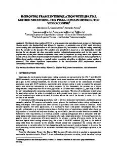
3. Spatial Interpolation on the Clouds We implemented three spatial interpolation methods: nearest neighbor, bilinear, and bicubic interpolation. We coded the three interpolation methods in C# and ran the code on the seven different Windows Server 2008 cloud instances available on Amazon EC2: T1 Micro, M1 Large, M1 XLarge, M2 Large, M2 2XLarge, M2 4XLarge, and C1 XLarge. The details of the configuration of the seven instances are given in Table 1. To test the performance of spatial interpolation on the different types of instances, we considered a large input point file of about 100 million elevation points distributed on a grid of 5000 x 19483 points. The input file size is 1.27 GB. Figure 1 shows the performance (execution time) of the three interpolation algorithms on the seven cloud instances. The figure shows that there is a clear outlier amongst the seven instances, namely, the T1 Micro instance. The low performance in this case indicates that, in practice, it is not useful to use this instance for data- and computeintensive applications. Figure 2 shows the same performance results as in Figure 1 but without the case of the T1 Micro instance. The figure shows that, for all cases, the M2 4XLarge instance gives the best performance. The figure also shows that the performance difference is almost negligible between the three instances M2 XLarge, M2 2XLarge, and M2 4XLarge. The explanation to this is that the code of the application is not able to exploit the added computing resources. Spatial interpolation is a highly data parallel computation. Coding this computation using traditional programming schemes (nested loops) results in lowerthan-achievable performance. Because data independence is not properly exploited, some of the available cores remain idle while only some cores are processing the interpolation. We conducted experiments to assess the impact on performance when varying memory size and computing power. Figure 3 shows the impact of different memory sizes. The results show that, beyond a certain memory size, little improvement can be achieved by using cloud instances with larger memory. In this case, using cloud instances with memory sizes larger than 17.1 GB would have little impact on performance. In practice, scientists could use such a result to select a cloud instance with a memory size that is most appropriate to the application at hand. The memory threshold depends on several parameters (computational behavior of the application, type of the operating system used, number of cores used and size of their cache, etc.). We argue that, for any specific application, it could be necessary to conduct a set of preliminary “trial-and-error” experiments to determine the appropriate memory threshold to use for the actual deployment. We also studied the impact on performance when changing the number of virtual cores (as defined in EC2). Figure 4 shows that using more computing power does not always improve performance. In this case, using instances with more than 13 virtual cores would not reduce the execution time substantially. For example, consider the case of bicubic interpolation. With an instance of 13 virtual cores (M2 2XLarge), the execution time is 187.3 seconds. With an instance having 26 virtual cores (M2 4XLarge), the execution time is 184.67 seconds. This is an improvement of only about 1.42%. In fact, increasing the number of virtual cores and decreasing memory may result in worse performance. For example, with an instance of 20 virtual cores (C1 XLarge), the execution time becomes 232.42 seconds. This is

due, in part, to the fact that the application’s memory Instance Type Memory Computing Power

requirements are much higher than its computing requirements. Storage API Name Cost (Windows Usage)

Micro Instance 32-bit or 64-bit platform I/O Performance: Low

613 MB

Up to 2 EC2 Compute Units

EBS storage only

t1.micro

$0.03 / hour

Large Instance 64-bit platform I/O Performance: High

7.5 GB

4 EC2 Compute Units (2 virtual cores with 2 EC2 Compute Units each)

850 GB of instance storage

m1.large

$0.48 / hour

Extra Large Instance 64-bit platform I/O Performance: High

15 GB

8 EC2 Compute Units (4 virtual cores with 2 EC2 Compute Units each)

1,690 GB of instance storage

m1.xlarge

$0.96 per hour

High-Memory Extra Large Instance 64-bit platform I/O Performance: Moderate

17.1 GB

6.5 EC2 Compute Units (2 virtual cores with 3.25 EC2 Compute Units each)

420 GB of instance storage

m2.xlarge

$0.62 / hour

High-Memory Double Extra Large Instance 64-bit platform I/O Performance: High

34.2 GB

13 EC2 Compute Units (4 virtual cores with 3.25 EC2 Compute Units each)

850 GB of instance storage

m2.2xlarge

$1.24 / hour

High-Memory Quadruple Extra Large Instance 64-bit platform I/O Performance: High

68.4 GB

26 EC2 Compute Units (8 virtual cores with 3.25 EC2 Compute Units each)

1690 GB of instance storage

m2.4xlarge

$2.48 / hour

High-CPU Extra Large Instance 64-bit platform I/O Performance: High

7 GB

20 EC2 Compute Units (8 virtual cores with 2.5 EC2 Compute Units each)

1690 GB of instance storage

c1.xlarge

$1.16 / hour

Table 1. Amazon EC2 Instances Used for Spatial Interpolation

Figure 1. Performance for Different Types of Instances

Figure 2. Performance for Different Types of Instances (Without the T1 Micro case)

Figure 5. Performance versus Cost Figure 3. Impact of Memory Size

Figure 4. Impact of the Number of Virtual Cores

3.1 Cost / Benefit Assessment Cost is a fundamental aspect when assessing whether cloud computing is a viable solution for geospatial science applications. We evaluated the performance obtained versus cost in the three types of interpolation. Figure 5 shows that, counter intuitively, using more expensive cloud instances does not necessarily mean better performance. Consider the case of bicubic interpolation. Using an instance with a cost of 0.48$/hour (M1 Large), the execution time was 294.96 seconds. When using an instance that is twice as expensive (M1 XLarge with 0.96$/hour), the execution time is 244.27 seconds. This is an improvement of only 20%.

4. Discussion As they mature, cloud platforms hold the key to solving many geospatial science problems requiring data- and computeintensive solutions. They enable scientists to choose the configuration that is most suitable to solve their science problem within their budget and time requirements. Our experiments showed a number of results related to several aspects:

Performance: Almost invariably, cloud computing provides an alternative that can be used successfully in many data- and compute-intensive Earth science applications. However, increasing the resources by using a cloud instance with more resources does not necessarily improve performance. In fact, it may be the case that performance degrades when using cloud instances with more resources. Performance obviously depends on how the application is designed. This is an issue also on traditional computing platforms (e.g., an on-premise cluster). However, in this case, users usually own their computing platforms and achieving sub-optimal performance on a given computing infrastructure is not a major issue. The challenge is to design and write applications so that they properly harness the memory, CPU cores, and levels of parallelism available on the clouds. Cost: Cloud computing provides a cost effective option to deploy data- and compute-intensive applications where results must be generated quickly. However, selecting the most cost effective cloud configuration for a given application may not be an easy task. Several test deployments must be evaluated to determine the most cost effective configuration. In the case of long running applications, we do not believe a cloud deployment is a good option in terms of cost. For example, if the interpolation application were a server application to be run for a year on an Amazon EC3 M2 XLarge instance, the cost to the application’s owner would be: 365 x 24 x 0.62 = $5431.2 which may be a prohibitively high cost. In this case, an on-premise deployment would be much more cost effective. Based on our experiments, we recommend that scientists carefully evaluate the actual needs of their applications before selecting cloud instances to run those applications. As shown earlier, more expensive instances with more resources may not necessarily translate into substantial improvements in terms of performance. Readers can find a detailed study about estimating the cost of a GIS in the Amazon cloud in ESRI (2011). Currently, there is no tool that systematically calculates the best cloud instance (in terms of both performance and cost) that scientists would have to select for a given application. Based on our experiments, we argue that geospatial scientists will have to consider the following two aspects:

Application Design and Management: In general, developing an application to be deployed on the clouds entails the same development effort as developing the same application to be deployed on a traditional on-premise server. Deploying existing applications on the clouds could be straightforward or could also be challenging. We argue that, in most cases, there are no development-related entry barriers for Earth scientists to deploy their applications on the clouds. Another conclusion is that Earth science applications that are inherently data parallel must be designed to properly exploit the availability of many CPU cores on the clouds. More importantly, we recommend that applications destined for the cloud be developed with the assumption of a dynamic number of CPU cores. This gives more flexibility when deploying the application on the cloud. Reliability: For the specific case of data- and compute-intensive geospatial applications, reliability1 is important only for the (few) scientists running an application on a given cloud platform, i.e., a failed execution impacts only a small number of users. However, in many cases, a geospatial application running on the cloud may be the background code for another (Web) application that is simultaneously accessed by a large number of users. In this case, reliability may be a crucial factor when evaluating the suitability of a given cloud-based solution. Given the higher reliability guarantees offered by cloud providers (compared to the reliability levels achievable through local servers), we argue that Earth scientists should consider cloud deployments for all applications with high reliability requirements. Figure 6 summarizes the typical decision flow to be considered when geospatial applications are considered for cloud deployment (Huang et al., 2010).

5. Future Research Cloud computing is now seen as a promising, cost-effective paradigm to support the execution of compute- and data-intensive geoscience applications. Experts in academia and in industry view it as a key enabler of data-intensive scientific discovery (Hey et al., 2009). Substantial research is still needed on how to best design geospatial applications to be efficiently executed on the clouds. We argue that, for geosciences to fully benefit from the emerging cloud computing paradigm, efforts will have to go into four directions: (i) developing new design approaches for geospatial applications specifically tailored for cloud environments, (ii) developing new mechanisms for accurate cost/benefit assessment of deploying applications on clouds, (iii) improving cloud platforms to better support geoscience applications, and (iv) exploring new distributed computing alternatives on the clouds. Application Design Approaches for the Clouds: As we discussed earlier, simply deploying geoscience applications onto cloud platforms may not necessarily improve their performance. This is particularly true in the case of highly data parallel tasks such as spatial interpolation. In these applications, performance improves only if the new computing resources are able to access data and avoid idling. A fundamental challenge in cloud applications is that, often, data are not co-located with computing 1

defined simply as the ability of the computing platform to properly run the application’s code and successfully generate the expected results.

resources (Armbrust et al., 2009). Network latencies may become the key element in determining an application’s overall performance. It is therefore crucial to carefully synchronize computations and data accesses so as to reduce the total execution time.

New Application

Legacy Application

Objective is Quick Deployment?

Source Code Available

No

Yes

Yes

Objective: Minimize Development Effort?

No

Application is Data Intensive?

Yes Rewrite as a CloudAware Code

Test Code on Cloud Instances with Different Configurations

Objective is Reducing Operational Cost

Yes

Consider Deploying on a Cloud MapReduce Cluster

Develop as a Cloud-Aware Code

Select a Cloud Instance with Moderate Memory Size and/or CPU Core Count (based on the testing results)

No

Objective is High Performance

Yes

No

Select A Cloud Instance with High CPU Core Count and/or Memory Size (based on the testing results)

Figure 6. Decision Flow for Deploying Geospatial Applications on the Clouds

Improving the Deployment Process: Deploying data- and compute-intensive applications on the cloud can be very costly. The deployment costs include the costs of deploying the application’s code and data onto the cloud and the cost of actually running the application, possibly for very long periods, on the cloud. Scientists must have mechanisms that accurately predict these costs. These decision making tools must consider a wide range of possibilities, e.g., hosting data on cloud A and code on cloud B, hosting data and code on the same cloud, hosting code only on a cloud and keeping data locally, etc. These tools will have to consider both the cost and the overall quality of the selected solution (performance, scalability, reliability, etc.) Improving Cloud Support to Geoscience Applications: A third direction is for cloud providers to better support geospatial applications with their typical characteristics (large volumes of geographic data, complex computations, need for visualization, etc.) Currently, most cloud providers offer generic services, user interfaces, and billing policies. These generic components must be adapted to better serve the needs of specific communities such as Earth scientists. For example, geoscience applications need to transfer massive amounts of geospatial data. Given that cloud

providers set fees for data transfer from/to their clouds, many geospatial applications would be very costly to deploy on clouds if their owners had to pay for data transfer at the same rates applied to other customers.

[10] Ghoshal D., R. Shane Canon, and Lavanya Ramakrishnan (2011), I/O Performance of Virtualized Cloud Environments, Proc. of the 2nd International ACM Workshop on Data Intensive Computing in the Clouds (DataCloud).

Exploring Distributed Computing Alternatives on the Clouds: Another potentially promising direction is to consider new distributed computing alternatives such as MapReduce, a framework that has proven to be adequate for applications that process massive amount of data (Dean and Ghemawat, 2004). Despite this success, little research has focused on exploring whether MapReduce can achieve the same levels performance for spatial applications. Recent work in this direction includes: Krishnan et al., 2010 and Akdogan et al., 2010.

[11] Hey T., S. Tansley, and K. Tolle (Eds) (2009), The Fourth Paradigm: Data-Intensive Scientific Discovery, Microsoft Research, ISBN 0982544200.

6. Acknowledgment This research is supported by NSF Project CSR-1117300, NASA SMD Cloud Computing Test Initiative NNX07AD99G, and the ESIP Cloud Testbed Initiative.

7. References [1] Akdogan, A.; Demiryurek, U.; Banaei-Kashani, F.; Shahabi, C.; Voronoi-Based Geospatial Query Processing with MapReduce, (2010). Proc. of the 2nd IEEE Intl. Cloud Computing Technology and Science(CloudCom), Indianapolis, IN, Nov. 30-Dec. 3. [2] Armbrust, M., Armando Fox, Rean Griffith, Anthony D. Joseph, Randy H. Katz, Andrew Konwinski, Gunho Lee, David A. Patterson, Ariel Rabkin, Ion Stoica, Matei Zaharia (2009), Above the Clouds: A Berkeley View of Cloud Computing, Technical Report No. UCB/EECS-2009-28, University of California at Berkeley, February. [3] Blower, J. (2010). GIS in the Cloud: Implementing a Web Map Service on Google App Engine. In Proc. of the 1st Intl. Conf. on Computing for Geospatial Research & Applications, Washington D. C., June. [4] Collins James P. (2010), Sailing on an Ocean of 0s and 1s, Science, Vol. 327 no. 5972 pp. 1455-1456. [5] Cornillon, P. (2009). Processing Large Volumes of SatelliteDerived Sea Surface Temperature Data - Is Cloud Computing the Way to Go? In Proc. of the Workshop on Cloud Computing and Collaborative Technologies in the Geosciences, Indianapolis, IN, September 17-18. [6] Dean J. and S. Ghemawat (2004). MapReduce: Simplified Data Processing on Large Clusters. OSDI, pp. 137-150. [7] ESRI (2011). Estimating the Cost of a GIS in the Amazon Cloud. [8] ESRI (2010). ArcGIS and the Cloud. http://www.esri.com/technology-topics/cloudgis/arcgis-andthe-cloud.html. [9] Evangelinos C. and Chris N. Hill (2008). Cloud Computing for Parallel Scientific HPC Applications: Feasibility of Running Coupled Atmosphere-Ocean Climate Models on Amazon’s EC2, Proc. of the 1st Workshop on Cloud Computing and its Applications (CCA), Chicago, IL, October 22–23.

[12] Hill, C. (2009). Experiences with Atmosphere and Ocean Models on EC2. In Proc. of the Workshop on Cloud Computing and Collaborative Technologies in the Geosciences, Indianapolis, IN, September 17-18. [13] Huang Q., Yang C., Nebert D., Liu K., Wu H. (2010) Cloud Computing for Geosciences: Deployment of GEOSS Clearinghouse on Amazon’s EC2. In proceedings of ACM SIGSPATIAL International Workshop on High Performance and Distributed Geographic Information Systems (HPDGIS), November, San Jose, CA. [14] Kim, K. S., and MacKenzie, D. (2009). Use of Cloud Computing in Impact Assessment of Climate Change. In Proc. of the Free and Open Source Software for Geospatial (FOSS4GT), Sydney, Australia, October 20-23. [15] Krishnan, S.; Baru, C.; Crosby, C. (2010); Evaluation of MapReduce for Gridding LIDAR Data, Proc. of the 2nd IEEE Intl. Cloud Computing Technology and Science (CloudCom), Indianapolis, IN, Nov. 30 2010-Dec. 3. [16] Liu, K., Yang, C., Li, W., Li, Z., Wu, H., Rezgui, A., & Xia, J. (2011). The GEOSS Clearinghouse High Performance Search Engine. The 19th International Conference on Geoinformatics, June 24-26, Shanghai, China. [17] McEvoy, G. V., and B. Schulze (2008): Using Clouds to Address Grid Limitations, Proc. of the 6th International Workshop on Middleware for Grid Computing (MGC), Leuven, Belgium, December 1-5. [18] Omnisdata (2010). GIS Cloud Beta: The Next Generation of GIS. http://www.giscloud.com. [19] Xie, J., Yang, C., Zhou, B., and Huang, Q. (2010). High Performance Computing for the Simulation of Dust Storms. Computers, Environment, and Urban Systems, 34(4):278290. [20] Yang C., Goodchild M., Huang Q., Nebert D., Raskin R., Bambacus M., Xu Y., Fay D. (2011a). Spatial Cloud Computing – How Can Geospatial Sciences Use and Help to Shape Cloud Computing, International Journal of Digital Earth, 4(4), 305-329. [21] Yang C., Wu H., Huang Q., Li Z., and Li J. (2011b) Using Spatial Principles to Optimize Distributed Computing for Enabling the Physical Science Discoveries, Proc. of the National Academy of Science. [22] Wang, Y., Wang, S., and Zhou, D. (2009). Retrieving and Indexing Spatial Data in the Cloud Computing Environment. In Proc. of the 1st International Conference on Cloud Computing, Beijing, China, December 1-4, Lecture Notes in Computer Sciences, Vol. 5931, pages 322-331.