Spatial Interpolation Using Neural Fuzzy Technique Kok Wai Wong1 , Tamás D. Gedeon1 , Chun Che Fung2 , Patrick M. Wong3 1
School of Information Technology Murdoch University Western Australia Email: { kwong | t.gedeon }@murdoch.edu.au 2
School of Electrical and Computer Engineering Curtin University Western Australia Email:
[email protected] in.edu.au 3
School of Petroleum Engineering University of New South Wales Sydney, Australia Email:
[email protected]
Abstract: Spatial interpolation is an important feature of a Geographic Information System, which is the procedure used to estimate values at unknown locations within the area covered by existing observations. This paper constructs fuzzy rule bases with the aid of a Selforganising Map (SOM) and Backpropagation Neural Networks (BPNNs). These fuzzy rule bases are then used to perform spatial interpolation. A case based on the 467 rainfall data in Switzerland is used to test the neural fuzzy technique. The SOM is first used to classify the data. After classification, BPNNs are then use to learn the generalization characteristics from the data within each cluster. Fuzzy rules for each cluster are then extracted. The fuzzy rules base are then used for rainfall prediction.
1. INTRODUCTION In a Geographic Information System (GIS), spatial interpolation is an essential feature [1]. Normally, points with known values are used to estimate values at other points. All spatial interpolation techniques can be grouped into global and local methods [1]. In a global method, all the information available is used to estimate an unknown value, while local methods only use a sample of the information for estimation. However, in [2], the authors have discussed the functionality of local method and found that they provide better results as compared to global method. Therefore, in this paper, the analysis will be based on local methods. In a global method, trend surface analysis is normally performed. The equation that can be used to estimate values at other points using a third-order trend surface is: Z= b 0 + b1 X + b2 Y + b 3 X 2 + b 4 XY + b5 Y 2 + b 6 X 3 + b 7 X 2 Y + b8 XY
2
+ b9Y 3 (1)
where b coefficients are estimated from the available information points. Equation (1) can also be written as: Z = f (X,Y)
(2)
As for a local method, the spatial interpolation of the value Z i in the i- th surface is: Z i = f ( X i , Yi )
(3)
Artificial Neural Networks (ANNs) have emerged as an option for spatial data analysis [2,3]. The observation sample that is used to derive the predictive model is known as training data in an ANN development. The independent variables, or the predictor variables, are known as the input variables and the dependent variables, or the responses, are known as the output variables. ANN analysis is quite similar to statistical approaches in that both have learning algorithm to help them realise the data analysis model. However, an ANN has the advantages of being robust with the ability to handle large amounts of data. Novice users can also easily understand the practical use of an ANN. An ANN also has the ability to handle very complex functions [4]. The main limitation of using ANN is that the data analysis model built may not be able to be interpreted. Fuzzy logic is also becoming popular in dealing with data analysis problems that are normally handled by statistical approaches or ANNs [5]. However, conventional fuzzy system systems do not have any learning algorithm to build the analysis model. Rather, they make use of human knowledge, past experience or detailed analysis of the available data by other means in order to build the fuzzy rules for the data analysis. The advantages of using fuzzy system are the ability to interpret the analysis model built and to handle
vagueness and uncertainty in the data. The data analysis model can also be changed easily by modifying the fuzzy rule base. The major limitation is the difficulty in building the fuzzy rules due to lack of learning capability. ANNs and fuzzy logic are complementary technologies in designing an intelligent data analysis approach [6]. That suggests combining the two [7]. For example, fuzzy logic could be used to enhance the performance of the neural network. In another approach, a neural network and fuzzy system could be integrated into a single architecture. However, a human analyst may still have difficulties understanding the analysis model computed. Analysis of the prediction model is also very time consuming. Therefore, it is one of the prime objectives of this paper to find a better way of combining the advantages of the ANN and fuzzy logic such that it can be used in spatial interpolation problem. 2.
NEURAL FUZZY SPATIAL INTERPOLATION
ANN and fuzzy logic are complementary technologies for the designing of spatial interpolation tools. However, there are many ways that the combination can be implemented [7]. Table 1 shows the different ways that ANN and fuzzy system can work together. It is important to observe the characteristics under each class so as to determine the appropriate technique that the analyst will be comfortable with. Table 1: Different ways to combine ANN and fuzzy logic Techniques Description Fuzzy Neural Use fuzzy methods to Networks enhance the learning capabilities or performance of ANN Concurrent Neuro- ANN and Fuzzy Fuzzy systems work together on the same task without any influence on each other Cooperative Neuro- Use ANN to extract Fuzzy rules and then it is not used any more Hybrid Neuro-Fuzzy ANN and Fuzzy are combined into one homogeneous architecture The Cooperative Neuro-Fuzzy technique is selected as the more appropriate technique to be used in this application. The reasons are as follow. As the BPNN can generalise from the data through some learning algorithm, the spatial interpolation
function could be realised automatically. This will also enable the fuzzy rules to cover the whole universal of discourse, so that they can be used to approximate data that are not present in the training set. As fuzzy rules are closer to human reasoning, the analyst could understand how the interpolation model performs prediction. If necessary, the analyst could also make use of his/her knowledge to modify the interpolation model. A. Clustering using self-organizing map For local spatial interpolation, the first step is to classify the available data into different classes so that the data are split into homogeneous subpopulations. Self-organizing Map (SOM) [8] is used to divide the data into sub population and hopefully reduce the complexity of the whole data space to something more homogeneous. The objective in this step is to make use of an unsupervised learning algorithm to sub-divide the whole population. The SOM is selected for this purpose mainly because it is a fast, easy and reliable unsupervised clustering technique. Let the input data space ℜn be mapped by the SOM onto a two-dimensional array with i nodes. Associated with each i node is a parametric reference vector mi =[µi1 ,µi2 ,… ,µi2 ]T ∈ ℜn , where µij is the connection weights between node i and input j. Therefore, the input data space ℜn consisting of input vector X=[x1 ,x2 ,..,xn ]T, ie X ∈ ℜn , can be visualized as being connected to all nodes in parallel via a scalar weights µij . The aim of the learning is to map all the n input vectors Xn onto mi by adjusting weights µij such that the SOM gives the best match response locations. SOM can also be said to be a nonlinear projection of the probability density function p(X) of the high dimensional input vector space onto the twodimensional display map. Normally, to find the best matching node i, the input vector X is compared to all reference vector mi by searching for the smallest Euclidean distance || X – mi ||, signified by c. During the learning process the node that best matches the input vector X is allowed to learn. Those nodes that are close to the node up to a certain distance will also be allowed to learn. The learning process is expressed as: m i (t + 1) = m i ( t) + h ci (t )[ X ( t) − m i (t )] (4) where t is discrete time coordinate and hci(t) is the neighbourhood function After the learning process has converged, the map will display the probability density function p(X) that best describes all the input vectors. At the end
of the learning process, an average quantisation error of the map will be generated to indicate how well the map matches the entire input vectors Xn . The average quantisation error is defined as: E = ∫ || X − m c || 2 p ( X ) dX
(5)
After the 2-dimensional map has been trained, the reference vectors that were used in the nodes of the map can be also obtained. In spatial interpolation, the reference vector will be the node center and consists of the input variables (x, y) and the output variable (z). As we like the clusters to be formed to facilitate the concept used in Euclidean interpolation, we propose here to construct the clustering boundaries based on the output reference vector of the nodes. The rule of thumb for deciding on the clustering boundaries is to examine the distance measure between the neighboring reference values. If the distance measure between the present reference node and the neighboring nodes is high, that suggests another cluster. B. Trend surface analysis using backpropagation neural networks After the set of available training data has been subdivided, BPNNs are trained in each cluster to predict only data within the cluster. Therefore, if the SOM identified c clusters, then c BPNNs need to be trained. When a BPNN [9] is used in spatial analysis, the observations obtained from the neighbouring are used as the training data, thus it is a supervised learning technique. The input neurons of the BPNN in this case correspond to the x and y position coordinates, and the output neuron is assigned to the variable that we want to perform spatial interpolation. The BPNN has a number of layers. The input layer consists of all the input neurons and the output layer just the output neuron. There are also one or more hidden layers. All the neurons in each layer are connected to all the neurons in next layer with the connection between two neurons in different layers represented by a weight factor. After the BPNN has learned and generalised from the training data, it is then used to construct the fuzzy rules bases. C. Knowledge representation using fuzzy rules As all the BPNNs have generalized from the training data, the next step is to extract the knowledge learned by the BPNNs. In this case, it is the same as the previous section; we will have to extract c fuzzy rule bases. The following algorithm outlines the steps in extracting the fuzzy linguistic rules for one BPNN.
As we have to extract fuzzy rules that can cover the whole universal of discourse in order to cover the whole sample space as seen by the BPNN, for T membership functions or linguistics terms, we would have T2 fuzzy rules as we have only two variables (x, y) in this case. We randomly generate input variables that could cover all the possible input space as seen by the BPNN and input it into the BPNN to obtain the rainfall measurements predicted by the BPNN. For the two inputs (x, y), the BPNN generates input (x, y)-output (z) data pairs with n patterns: ( x n , y n; zn ) The number of linguistics terms T used in this fuzzy rule extraction has to be the same as the predetermined one when generating output from the BPNN. The distribution of the membership functions in each dimension of the domain in this case is evenly distributed. For ease of interpolation and computational simplicity, the shape of the membership functions used in this rule extraction technique is triangular. In this case, we will obtain for every x ∈ X , At : X → [ 0,1 ]
(6)
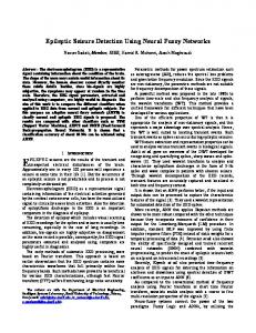
After the fuzzy regions and membership functions have been distributed, the available in put-output pairs will be mapped. If the value cuts on more than one membership function, the one with the maximum membership grade will be assigned to the value: R n ⇒ [ x n ( Ax , max), y n ( A y , max) : z n ( B z , max)] (7) After all the input-output values have been assigned a fuzzy linguistic label, Mamdani type fuzzy rules are then formed [10]. After the fuzzy rules base corresponding to the BPNN for a class have been constructed, the BPNN is not used anymore when performing spatial interpolation. With this set of fuzzy rules, a human analyst can now examine the behaviour of the interpolation. Changes and modification can then be performed if necessary. The fuzzy rules extracted can also handle fuzziness in the data and thus may improve the performance of the spatial interpolation. Figure 1 shows the block diagram of establishing the spatial interpolation model and Figure 2 shows the block diagram of performing the spatial interpolation.
Figure 1: Establishing the spatial interpolation model
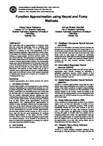
Figure 2: Performing spatial interpolation from the fuzzy rules bases 3. CASE STUDY AND DISCUSSION In this case study, the data from [2] is used. The data is collected on 8th May 1996 in Switzerland. 100 data locations are used as the training data and the other 367 locations data are then used to verify the prediction accuracy of the established spatial interpolation model. The two input variables used in this case is the 2D coordinate position (x, y); and the output used is the rainfall measurements (z). The digital elevation model (DEM) (v) is also available but was not used in the case study as in [2]. The 100 training data points are fed into the SOM for unsupervised clustering. After performing the cluster boundaries determination, the classes are formed. Before being input into individual BPNNs, the data needs to be normalized between 0 and 1. Linear normalization is used with maximum and minimum vales unique to the class. In this case, the SOM identified a total of 8 classes. After the data has
been normalized, 8 BPNNs are trained to handle their own sub-populations. After examining the maximum and minimum value of each class, the appropriate number of membership function used is determined to be 7. In this case, the number of fuzzy rules extracted for each BPNN (each class) is 49, i.e. 72 . With the distribution information for each linguistic term, the user can easily understand the set of fuzzy rules and understand how the prediction is performed. The results of this technique are compared to the results obtained from [2] as tabulated in Table 2 by using mean absolute error (MAE): MAE =
1 n * ∑ zi − zi n i =1
(8)
and root mean square error (RMSE): RMSE =
1 n * ∑ (z i − z i ) 2 n i =1
(9)
Table 2: Comparisons of results Technique MAE RMSE Neural 53.86 72.95 Technique Technique used 55.9 78.6 in [2] This neural fuzzy technique has performed better than the technique used in [2] with the advantage of understanding the underlying function of the BPNNs with a set of fuzzy rules. With the sets of fuzzy rules, human analyst can modify and add-on knowledge to enhance the model. As individual fuzzy rule sets are constructed for each individual cluster, analyst can have a better understanding in the feature of that cluster. 4. CONCLUSION This technique uses SOM to divide the data into sub population and hopefully reduce the complexity of the whole data space to something more homogeneous. After the classification boundaries have been identified, the whole training data set is then sub-divided into the respective classes. BPNNs corresponding to each individual class are then trained using the cross-validation approach. After all the BPNNs have been trained, fuzzy rule bases for each class are then constructed. The case study used has shown that this method can produce better results as compare to the technique used in [2]. Beside, the advantages of using this technique are as follows. First it makes use of the robustness and learning ability of the ANN to sub-divide and generalize from training data. After which, the learned underlying function is then translated into fuzzy rules. With the use of fuzzy rules, the interpretability and the ability of handling vagueness and uncertainty has enhanced the interpolation model. 5. ACKNOWLEDGMENT This research is supported by the Australian Research Council REFERENCES 1.
2.
Burrough, P., and McDonnell, R. Principles of geographical information systems, Oxford University Press, New York, (1998). Lee, S., Cho, S., and Wong, P.M. “Rainfall prediction using artificial neural network”, Journal of Geographic Information and
Decision Analysis, vol. 2, no. 2 (1998) 254264. 3. Friedman, J.H. “An Overview of Predictive Learning and Function Approximation”, From Statistics to Neural Networks: Theory and Pattern Recognition Applications, SpringerVerlag (1994) 1-61. 4. Cherkassky, V., Friedman, J.H., and Wechsler, H. From Statistics to Neural Networks: Theory and Pattern Recognition Applications, Springer-Verlag (1994). 5. Kosko, B. Fuzzy Engineering, Prentice-Hall (1997). 6. Williams, T. “Special Report: Bringing Fuzzy Logic & Neural Computing Together”, Computer Design, July (1994), 69-84. 7. Nauck, D. “Beyond Neuro-Fuzzy: Perspectives and Directions”, Proceedings of the Third European Congress on Intelligent Techniques and Soft Computing, (1995) 1159-1164 8. Kohonen, T. "The Self-Organising Map", Proceedings of the IEEE, Vol. 78, No. 9, September (1990) 1464-1480. 9. Rumelhart, D.E., Hinton, G.E. and Williams, R.J. "Learning Internal Representation by Error Propagation" in Parallel Distributed Processing, vol. 1, Cambridge MA: MIT Press, (1986) 318-362. 10. Mamdani, E.H. and Assilian, S “An experiment in linguistic synthesis with a fuzzy logic contoller,” International Journal of ManMachine Studies, (1975) 1-13.