Proceedings of 2015 IEEE International Conference on Mechatronics and Automation August 2 - 5, Beijing, China
Spatial Linear Path-Following Control for an Underactuated UUV Zheping Yan, Haomiao Yu, Jiajia Zhou and Benyin Li College of Automation Harbin Engineering University Harbin, Heilongjiang Province, China
[email protected] three-dimensional space. In recent years, some researchers have increasingly concerned about the spatial linear pathfollowing based on the way-point guidance [3, 8-10]. However, these outcomes are presented based on the accurate dynamic models of UUVs. In the engineering, the accurate motion models of UUVs are unobtainable, since these hydrodynamic coefficients appear parameter perturbation when the vehicles sailing free surface or seafloor. Moreover, the measured values for these hydrodynamic coefficients are inaccuracy. Therefore, the motion control laws in the practice are required to be robustness with parameter uncertainties. In addition, owing to these vehicles sailing in the ocean be subject to the wave and current, these motion control laws are also asked to reject those external disturbances. In this work, the spatial linear path-following control problem of an underactuated UUV is discussed in detail, and a robust path-following control law is developed using the Lyapunov’s direct method and backstepping technique. The desired path is pre-planned based way-point guidance, and the path-following guidance law is established based on line of sight (LOS), Serret-Frenet frame and the “virtual vehicle” method. This guidance law can effectively reduce the amount of calculation. To eliminate parameter perturbation, the upper bound of the parameter perturbation is introduced to design the dynamic path-following control law. Moreover, a nonlinear tracking differentiator is introduced into the loop of the surge velocity control, which can effectively avoid setpoint jump and chattering. Based on the Lyapunov’s stability theory, this control law can globally exponentially stabilize all state errors. The organization of the remainder of the paper is as follows. Section 2 describes the six DOF motion model of an underactuated UUV sailing in the three-dimensional space. Section 3 provides the path planning and the guidance law based on the “virtual vehicle” method and way-points guidance method. In section 4, the spatial path-following control law is developed by using the Lyapunov’s direct method and backstepping technique. The numerical simulation results and discussion are reported in section 5. At last, section 6 provides conclusions. II. UUV MOTION MODEL
Abstract - The problem of three-dimensional linear pathfollowing for an underactuated UUV is addressed. The pathfollowing guidance law is established by using line of sight (LOS), Serret-Frenet frame and the “virtual vehicle” method. For surge velocity control, steering control and diving control, three dynamic control laws are provided by using the Lyapunov’s direct method and backstepping technique, respectively. It is easy proven that this control scheme can force all state errors to globally exponentially converge to zeros. At last, a series of simulation results are provided to illustrate strongly robust and preferably control performance of this control scheme. Index Terms - Underactuated UUV, way-point, line of sight, spatial linear path-following control, globally exponentially stable.
I. INTRODUCTION With the deepening marine development, unmanned undersea vehicle (UUV) has been extensively applied in various fields of marine engineering and marine defense, such as ocean resource assessment, inspection of underwater structures, seafloor mapping, submarine rescue, and so on [1]. To achieve the above-mentioned missions, these vehicles must be required precise guidance and control. In practice, the desired path is described as a series of way-points, that is, the connection between two adjacent way-points represents the desired path. These way-points are beforehand stored in a database onboard vehicle, which is generated using substantial criteria like mission, weather conditions, obstacles, collision avoidance, and so on [2-4]. It is typically desired that the undersea vehicle follows the connection as close as possible. The problems of the path-following control for UUV is extremely challenging because the vehicle is highly nonlinear, parameter perturbation and unmeasured disturbance. Moreover, considering the economic, safely and efficiency, these vehicles possess less independent control inputs than degrees-of-freedom. Brockett’s theorem deems that there do not exist any continuous time-invariant feedback control law to asymptotically stabilize the underactuated UUV dynamics [5]. In the practice, the way-point guidance has been broadly adopted in wheeled mobile robots, surface ships and undersea vehicles [2, 3, 6-10]. For these scenarios, it is typically used the guidance and control in the context of cross-track control or linear path following. In these aforementioned works, the horizontal path-following is still the core issue [2, 6, and 7]. Furthermore, some works in the horizontal curvilinear pathfollowing are also presented in succession [11-13]. However, the undersea vehicles are six degrees of freedom (DOF) in the 978-1-4799-7098-8/15/$31.00 ©2015 IEEE
This section describes the kinematic and dynamic model of motion of an underactuated UUV moving in the threedimensional space. These motion equations are presented by using standard notation [4]. The independent control inputs
139
are the surge force, the pitch and yaw torque provided by the aft thrusters. The model details are obtained in [4]. A. Kinematics To describe the rigid-body kinematics, the inertial reference frame {I} and a body-fixed frame {B} are employed, see Fig.1. The origin of {B} frame coincides with the midpoint of the UUV center of mass (CM) and the center of buoyancy (CB). In the guidance and control applications, it is usually to use the xyz convention (roll-pitch-yaw), which is defined in terms of Euler angles or quaternions. Therefore, the kinematic equations of an underactuated UUV take the form ξ = u cosψ cos θ + v(cosψ sin θ sin φ − sinψ cos φ ) (1a) + w(cosψ sin θ cos φ + sinψ sin φ ) η = u sinψ cos θ + v(sinψ sin θ sin φ + cosψ cos φ ) (1b) + w(sinψ sin θ cos φ − cosψ sin φ )
ζ = −u sin θ + v cos θ sin φ + w cos θ cos φ
(1c)
φ = p + q sin φ tan θ + r cos φ tan θ
(1d)
m55 q = (m33 − m11 )uw + (m66 − m44 ) pr − M q q − M q q q q − ( zGW − z B B) sin θ + τ 5 m66 r = (m11 − m22 )uv + (m44 − m55 ) pq − Nr r − Nr r r r + τ 6
K ( i ) , M ( i ) and N ( i ) capture hydrodynamic damping effects;
τ 1 , τ 5 and τ 6 denote the surge force, the pitch and yaw torque provided by the aft thrusters. Note that the equation for v , w and q in (2b, c and d) do not exist any external control input. III. PATH PLANNING AND GUIDANCE A
Path Planning Considering an underactuated UUV described Eqs. (1-2), the predefined path is obtained by sequentially linking a series of way-points {WP1 , WP2 ,… ,WPi ,… ,WPn } stored in a database. Each way-point can be described using Cartesian coordinates WPi = ( xi , yi , zi ) for i = 1,…… , n [4].Hence, the waypoint database consists of wpt.pos = {( x1 , y1 , z1 ), ( x2 , y2 , z 2 ),… , ( xn , yn , zn )} (3)
of the {B} with respect to the {I}; u , v and w state the linear velocity; p , q and r express the angular velocity.
Let Li −1 denote straight segment between way-point WPi −1 and WPi . In this task, it is generally assumed that the surge velocity of the vehicle is constant and positive and there are bounds on all angular velocity q and r . The way-point WPi
The inertial reference frame {I}
y v
E
φ
ξ
ψ
ζ
q
τ
pitch
sway
p
τ
τ
roll
x
u
6
is chosen as the turning point from path Li −1 to Li . The turning strategy takes the form: when the vehicle sails to a spherical neighborhood whose center of sphere is way-point WPi and radius of sphere is Ri , the desired path of the UUV
1
τ
1
switches to the next straight segment Li , the starting point and 5
destination of which are way-point WPi
w
r
z The body-fixed reference frame {B} Fig. 1. The vehicle motion states, the inertial reference frame {I} and the body-fixed reference frame {B}.
B. Dynamics For control design tasks, it is generally assumed that (I) the mass distribution is homogeneous; (II) the hydrodynamics drag terms of order higher than two are neglected; (III) the vehicle is a neutrally buoyant and the shape structure is approximately symmetrical. The dynamic model of an underactuated UUV moving the three-dimensional space expressed by the following differential equations [4, 14] m11u = m22 vr − m33 wq − X u u − X u u u u + τ 1 (2a) m22 v = m33 wp − m11ur − Yv v − Yv v v v
(2b)
m33 w = m11uq − m22 vp − Z w w − Z w w w w
(2c)
m44 p = (m22 − m33 )vw + (m55 − m66 )qr − K p p − K p p p p
and WPi +1 ,
respectively. In the straight segment Li , therefore, the predefined path is parameterized as ⎧ xd,i ( s ) = kix s + xi ⎪ y (4) ⎨ yd,i ( s ) = ki s + yi ⎪ z (s) = k z s + z i i ⎩ d,i
surge
− ( zGW − z B B) cos θ sin φ
(2f)
where, mkk ( k = 1,… , 6 ) denote the inertia quantity including mass and hydrodynamic added mass term; X ( i ) , Y( i ) , Z ( i ) ,
θ = q cos φ − r sin φ (1e) ψ = q sin φ / cos θ + r cos φ / cos θ (1f) where, ξ , η and ζ denote the coordinate components of the CM of the vehicle in the {I}; φ , θ and ψ are the orientation
η θ
(2e)
where, s ∈ [ 0,1] ; k x ,i , k y ,i and k z ,i are the direction numbers
of the predefined path, and their definitions are as following: ⎧ kix = xi +1 − xi ⎪ y (5) ⎨ ki = yi +1 − yi ⎪k z = z − z i +1 i ⎩ i B Guidance To perform spatial path-following tasks, the appropriate guidance law is established by using LOS and the “virtual vehicle” method, see Fig.2. A series of the local Serret-Frenet frames are introduced on the way-point WPi for i = 1,… , n − 1 , respectively. The way-point WPi is the origin of the relevant
(2d)
local Serret-Frenet frame {Fi}. Its xF ,i − axis coincides with
140
⎧υ1 = υ2 ⎪ υ 2 υ2 ⎨ ) ⎪υ2 = − R sgn(υ1 − ud + ⎩ 2R where, ud is the desired surge velocity.
the straight segment Li . These local frames {Fi} can be obtained by rotating the inertial coordinate frame {I} translated to the way-point WPi to angle ψ iF and θiF about the Eζ − axis and Eη − axis, respectively. These rotation angles are defined as zi +1 − zi θiF = − arctan( ) (6a) ( xi +1 − xi ) 2 + ( yi +1 − yi )2
η
A
z F , i +1
Δψ Δθ
yF , i
xF , i
B C
{Fi}
WPi −1 {Fi-1}
z F ,i −1
WPi zF ,i
O
{Fi+1}
For simplifying the controller design, the rolling motion may be neglected, that is, φ = φ = 0 , p = p = 0 . Moreover, the six-degrees-of-freedom motion model of an underactuated UUV is divided into three noninteracting subsystems: surge velocity control, steering and diving. And then, using the Lyapunov’s direct method and backstepping technique, three control laws are developed to track the desired surge velocity, pitch angle and yaw angle, respectively. And then, these control laws drive the vehicle to follow the desired path that is described a series of way-points in the database. A Surge Velocity Controller Considering the surge velocity control subsystem, the surge velocity error variable is defined as following ue = u − υ1 (14) The control objective of the surge velocity change how to stabilize the error variable ue . The Lyapunov function is
defined as following 1 m11ue2 (15) 2 Tacking the derivative of Eq. (15) and calling Eq. (2a), we V1 =
can obtain as following V1 = m11ue ue = (u − υ1 )(m11u − m11υ2 )
(11b)
= (u − υ1 )(m22 vr − m33 wq − X u u − X u u u u + τ 1 − m11υ 2 )
zeI → 0 ,
yeI → 0 . The desired pitch angle and yaw angle are
(16)
To ensure the derivative V1 to be negative with considering the parameter perturbation, the surge velocity control law is
θ d = θ + Δθ ψ d = ψ + Δψ (12) Right now, the control objectives change into adjust the attitude of the vehicle to align the desired pitch angle and yaw angle. And then, the vehicle sails to the pre-defined path with constant surge velocity along the desired course. To avoid setpoint jump and chattering, a nonlinear tracking differentiator is introduced to arrange the excessive process of the surge velocity of the vehicle [15]. The specific expression of this tracking differentiator is provided as following F i
xF ,i −1
IV. CONTROL LAW DESIGN
And then, substituting for sB in Eqs. (4), the coordinates of the point B can be calculated as ( xB , yB , z B ) = (kix sB + xi , kiy sB + yi , kiz sB + zi ) (8) The inertial position errors are defined as xeI = x − xB yeI = y − yB zeI = z − z B (9) Thus, the position errors variables in the {Fi} frame are calculated as ⎡ xeF ⎤ ⎡ cosψ iF cos θ iF sinψ iF cos θ iF − sin θiF ⎤ ⎡ xeI ⎤ ⎢ F⎥ ⎢ ⎥⎢ ⎥ F cosψ iF 0 ⎥ ⎢ yeI ⎥ (10) ⎢ ye ⎥ = ⎢ − sinψ i ⎢ zeF ⎥ ⎢ cosψ iF sin θiF sinψ iF sin θ iF cos θ iF ⎥ ⎢ zeI ⎥ ⎣ ⎦ ⎣ ⎦⎣ ⎦ According to the geometrical relationship in Fig. 2, the angles of the LOS are defined as zeF Δθ = − arctan( ) (11a) l 2 + yeF 2
⇒
E
Fig. 2. The schematic 3D path-following of an UUV based on way-points guidance and LOS.
( x, y, z ) denote the position coordinates of the vehicle in the {I} frame. According to the geometrical relationship in Fig. 2 and the principles of LOS, the parameter coordinate s of the point B is solved as k x ( x − x) + kiy ( yi − y ) + kiz ( zi − z ) sB = − i i (7) kix 2 + kiy 2 + kiz 2
yeF ) l Eqs. (11) indicate that Δθ → 0 , Δψ → 0
WPi +1
yF ,i −1
ζ
xF ,i +1 yF ,i +1 l = k LOS L0
point of the vehicle. The distance l between points A and B is normally set at 2-5 times the total length L0 of the vehicle. Let
Δψ = arctan(
ξ
WPi + 2
yi +1 − yi (6b) xi +1 − xi Let point B represent the projection point of the origin O of the {B} on the straight segment Li and point A is the target
ψ iF = arctan
{I}
(13)
F i
chosen as
τ 1 = −mˆ 22 vr + mˆ 33 wq + Xˆ u u + Xˆ u u u u + mˆ 11υ2 − K1 K1 = m22 vr + m33 wq + X u u + X u u u 2 + m11 υ 2 + k1mˆ 11ue
(17a) (17b)
where, “^” denotes the nominal hydrodynamic coefficients; “~” denotes the upper bound of the parameters perturbations; k1 is positive constant gains to be chosen later.
141
From the definition of the Lyapunov function V3 , it is radially unbounded and satisfies the following inequality 1 2 2 [ψ e , re ] ≤ V3 ≤ (1 + mˆ 66 + m66 ) [ψ e , re ] 2 Theorem 3.4 in [16] indicates that the error ψ e and re globally exponentially converge to zero under the control
And then, the derivative V1 under the control law (17) satisfies the following inequality mˆ (18) V1 ≤ −k1mˆ 11 (u − υ1 ) 2 = −2k1 11 V1 m11 Moreover, the definition of the Lyapunov function V1 indicates that it satisfies condition of theorem 3.4 [16], that is, 1 1 2 2 (mˆ 11 − m11 ) ue ≤ V1 ≤ (mˆ 11 + m11 ) ue and it is radially 2 2 unbounded. Based on Theorem 3.4 in [16], the surge velocity error ue globally exponentially converges to zero
law (23). C
Diving Controller Similarly, the pitch angular error variable is defined as θe = θ − θ d . And then, the Lyapunov function is considered
1 V4 = θ e2 (25) 2 By ignoring the rolling motion, Eq. (1e) is simplified to θ = q . Tacking the derivative of Eq. (25), we can obtain as following: V4 = θ e (q − θ d ) . Considering the pitch angular velocity to be the virtual control input, the desired control law is chosen as qd = θ d − k4θ e (26) where, k4 is positive constant to be chosen later. In that way,
under the control law (17). B
Steering Controller For the steering controller design, the yaw angular error variable ψ e = ψ −ψ d is introduced to develop steering control law. The following control Lyapunov function is considered 1 V2 = ψ e2 (19) 2 Due to the rolling motion be neglected, Eq. (1f) is simplified to ψ = r / cos θ . And then, the derivative of Eq. (19) can be
The derivative V4 changes into V4 = − k4θ e2 + qeθ e , where qe = q − qd . Next, the Lyapunov function is provided to develop the dynamic diving controller. This Lyapunov function is defined 1 V5 = V4 + m55 qe2 (27) 2 Thus, the derivative of Eq. (27) is given V5 = V4 + m55 qe qe = −k4θ e2 + qe (θ e + m55 qe )
obtained V2 = ψ e (r / cos θ −ψ d ) . If the yaw angular velocity r is chosen as the virtual control input, the desired is set as rd = ψ d cos θ − k2ψ e cos θ (20) where, k2 is positive constant. Then, the derivative V2 changes into V2 = − k2ψ e2 + reψ e / cos θ , where re = r − rd . Calling Eq. (19), the following Lyapunov function is constructed as 1 V3 = V2 + m66 re2 (21) 2 Calculating the derivative of Eq. (21) and substituting for r in the derivative, we can obtain as following V3 = V2 + m66 re re = − k2ψ e2 + reψ e / cos θ + m66 re re
= −k2ψ + re (ψ e / cos θ + (m11 − m22 )uv 2 e
= −k4θ e2 + qe (θ e + (m33 − m11 )uw − M q q − M q q q q (28) − ( zGW − z B B)sin θ + τ 5 − m55 qd ) In order to reject the parameter perturbation, the diving
control law is chosen as τ 5 = (mˆ 11 − mˆ 33 )uw + Mˆ q q + Mˆ q q q q + ( zGW − z B B) sin θ
(22)
+ mˆ 55 qd − θ e − K 3
− N r r − N r r r r − m66 rd + τ 6 )
(29a)
Considering the parameter perturbation, the steering control
K 3 = (m11 + m33 ) uw + M q q + M q q q 2 + m55 qd + k5 mˆ 55 qe (29b)
law is set as τ 6 = (mˆ 22 − mˆ 11 )uv + Nˆ r r + Nˆ r r r r + mˆ 66 rd
where, k5 is positive constant to be chosen later. Under the control law (29), the derivative (28) turns into V5 = −k4θ e2 + qe (θ e + (m33 − m11 )uw − M q q − M q q q q
−ψ e / cos θ − K 2
(23a)
− ( zGW − z B B) sin θ + τ 5 − m55 qd )
K 2 = (m11 + m22 ) uv + N r r + N r r r 2 + m66 rd + k3 mˆ 66 re (23b)
= −k4θ e2 + qe (((m33 − mˆ 33 ) + (mˆ 11 − m11 ))uw − m55 qd
where, k3 is positive constant gains to be chosen later. In the role of the control law (23), the derivative (22) becomes V3 = −k2ψ e2 + re (ψ e / cos θ + (m11 − m22 )uv
+ ( Mˆ q − M q )q + ( Mˆ − M q q )q q + (mˆ 55 − m55 )qd − (m11 + m33 ) uw − M q q − M q q q 2 − k5 mˆ 55 qe )
− N r r − N r r r r − m66 rd + τ 6 ) = −k2ψ e2 + re (((mˆ 22 − m22 ) + (m11 − mˆ 11 ))uv + ( Nˆ r − N r )r + ( Nˆ r r − N r r )r r + (mˆ 66 − m66 )rd
(30)
≤ −k4θ e2 − k5 mˆ 55 qe2 ≤ − min(k4 , k5 mˆ 55 )(θ e2 + qe2 ) From the definition of the Lyapunov function V5 , it is radially unbounded and satisfies the following inequality 1 2 2 [θ e , qe ] ≤ V5 ≤ (1 + mˆ 55 + m55 ) [θ e , qe ] 2
(24)
− (m11 + m22 ) uv − N r r − N r r r 2 − m66 rd − k3 mˆ 66 re ) ≤ −k2ψ e2 − k3 mˆ 66 re2 ≤ − min(k2 , k3 mˆ 66 )(ψ e2 + re2 )
142
Theorem 3.4 in [16] indicates that the error θe and qe globally exponentially converge to zero under the control law (29). V. SIMULATION In this section, some simulation results are presented to illustrate the performance of the proposed path-following control law. In this simulation, the nominal values of these hydrodynamic coefficients of the vehicle are elaborated in [14]. In order to verify the effectiveness of the proposed pathfollowing control law, these simulation results are compared with the PID control law based on the LOS. The ±20% parameter uncertainty is introduced into this simulation, which is used to manifest the strong robustness in regard to the parameter perturbation. In this simulation, these control gain coefficients of the path-following control law are set as: R = 0.01 , k1 = 21.1 , k 2 = 0.5 , k3 = 15 , k4 = 8 and k5 = 5 . And then, the specific expression of the dynamic pathfollowing control law are Eqs. (17), (23) and (29). Considering the seabed exploration, the way-points in this simulation are planned as (m): WP1 = (80, 0,1) , WP2 = (80,180,10) , WP3 = (180,300,30) , WP4 = (180,500, 60) , WP5 = (100,500, 60) , WP6 = (100,300, 60) , WP7 = (50,300, 60) , WP8 = (50,500, 60) , WP9 = (0,500, 60) , WP10 = (0,300, 60) . The vehicle starts from rest, whose initial position is ξ (0) = 90 m , η (0) = 0 m , ζ (0) = 1 m and initial attitude is
Fig. 4. Time evolution of the position errors in the and
θ (0) = 0 ,ψ (0) = 0 . The desired surge velocity of the vehicle is set as 1 m/s. In Fig. 3-6, the simulation results under the proposed control law and PID are displayed. Figure 3 shows the three-dimensional scheme of the vehicle’s position together with the desired geometrical path. In Figure 3, from way-points WP1 to WP4 , the vehicle under the path-following control law based backstepping technique or PID performs diving mission, which is forced to the desired operating depth. And then, the vehicle executes specified operating mission from WP4 to WP10 . The vehicle is seem to follow the desired path high accuracy. The position errors are illustrated in Fig. 4.
ζ
ξ -direction, η -direction
-direction.
Fig. 5. Time evolution of the surge velocity and its scheduling instructions.
Fig. 6. Time evolution of the control signals τ 1 (t ) , τ 5 (t ) and τ 6 (t ) . From this figure, the position errors under PID based LOS exist high-frequency oscillation because of the parameter perturbation. Yet the proposed path-following control law can effectively stabilize the position errors. Figure 5 shows the time evolution of the surge velocity and its desired value. Though the traditional PID is simple, the settling time is longer than the proposed surge velocity controller. Figure 6 displays the time evolution of the control input.
VI. CONCLUSION
Fig. 3. Three-dimensional scheme of the measured and desired path during the simulation.
This article deals with the problem of the spatial linear path-following control of an underactuated UUV with the
143
parameter perturbation. The desired path is pre-mission programmed by using the way-point method. Then, the guidance law is established based on the “virtual vehicle” method. Next, a robust path-following control law is developed based the Lyapunov’s direct method and backstepping technique, which drive all state-errors to globally exponentially converge to zeros. These simulation results show that this control law is strong robust with the parameter perturbation and effectively achieve the threedimensional linear path-following. ACKNOWLEDGMENT This work is supported by National Natural Science Foundation (NNSF) of China under Grant 51179038 and 51309067. REFERENCES [1] J. Yuh, “Design and control of autonomous underwater robots: a survey,” Autonomous Robots, vol. 8, no.1, pp. 7-24, January 2000. [2] E. Fredriksen and K. Y. Pettersen, “Global κ -exponential way-point maneuvering of ships,” Proceedings of the 43rd IEEE Conference on Decision and Control, Atlantis, Paradise Island, Bahamas, December, 2004, pp. 5360-5367. [3] E. Borhaug and K. Y. Pettersen, “Adaptive way-point tracking control for underactuated autonomous vehicles,” Proceedings of the 44th IEEE Conference on Decision and Control, and the European Control Conference 2005, Seville, Spain, December, 2005, pp. 4028-4034. [4] T. I. Fossen, Handbook of Marine Craft Hydrodynamics and Motion Control, New York, USA: John Wiley and Sons Ltd, 2011, pp. 254-266. [5] R. W. Brockett, “Asymptotic stability and feedback stabilization,” Differential Geometric Control Theory, Boston: Birkhauser, 1983, pp. 181-191. [6] T. I. Fossen, M. Breivik, and R. Skjetne, “Line-of-sight path following of underactuated marine craft,” Proceedings of the 6th IFAC MCMC, Girona, Spain, 2003, pp. 244-249. [7] A. P. Aguiar and A. M. Pascoal, “Dynamic positioning and way-point tracking of underactuated AUVs in the presence of ocean currents,” International Journal of Control, vol. 80, no. 7, pp. 1092-1108, July, 2007. [8] E. Borhaug and K. Y. Pettersen, “Cross-track control for underactuated autonomous vehicles,” Proceedings of the 44th IEEE Conference on Decision and Control, and the European Control Conference 2005, Seville, Spain, December, 2005, pp. 602-608. [9] C. A. Woolsey and L. Techy, “Cross-track control of a slender, underactuated AUV using potential shaping,” Ocean Engineering, vol. 36, no. 1, pp. 82-91, January, 2009. [10]S. S. Bi, C. M. Niu, Y. R. Cai, L. G. Zhang, and H. X. Zhang, “A waypoint-tracking controller for a bionic autonomous underwater vehicle with two pectoral fins,” Advanced Robotics, vol. 28, no. 10, pp. 673-681, 2014. [11]L. Lapierre and D. Soetanto, “Nonlinear path-following control of an AUV,” Ocean Engineering, vol. 34, no. 11-12, pp. 1734-1744, 2007. [12]L. Lapierre and B. Jouvencel, “Robust nonlinear path-following control of an AUV,” IEEE of Oceanic Engineering, vol. 33, no. 2, pp. 89-102, 2008. [13]Zh. P. Yan, Y. B. Liu, J. J. Zhou, and D. Wu, “Path following control of an AUV under the current using the SVR-ADRC,” Journal of Applied Mathematics, 2014. [14]K. Y. Pettersen and O. Egeland, “Time-varying exponential stabilization of the position and attitude of an underactuated autonomous underwater vehicle,” IEEE Transactions on Automatic control, vol. 44, no. 1, pp. 112-115, January, 1999. [15]J. Q. Han, “From PID to active disturbance rejection control,” IEEE Transactions on Industrial Electronics, vol. 56, no. 3, pp. 900-906, March, 2009. [16]H. J. Marquez, Nonlinear Control Systems: Analysis and Design, New Jersey: John Wiley and Sons. Inc., 2003.
144