and evaluation, dynamic programming ... has been widely used in word recognition to com- pensate the ..... ming algorithm optimization for spoken word.
RESIDUAL COMPUTATION AND EVALUATION USING DYNAMIC TIME WARPING Francisco I. Gamero, David A. Llanos, Joan Colomer and Joaquim Mel´endez Grupo eXiT, University of Girona. Av. Lluis Santalo s/n E-17071-Girona (Spain) {gamero, dllanosr, colomer, quimmel}@eia.udg.es Abstract This work describes the adaptation of Dynamic Time Warping (DTW) algorithm in order to be used on-line for residual computation and evaluation purpose. The main motivation is to compensate modelling errors and characteristic hybrid systems behavior by using DTW. A laboratory plant has been used to test this approach. Keywords: Fault diagnosis, residual computation and evaluation, dynamic programming
1
INTRODUCTION
Fault Detection and Isolation (FDI) methods based on analytical redundancy (Chow and Willsky 1984) are widely used to diagnose systems whose mathematical model is available. The task of FDI is typically accomplished in two steps, namely residual generation and residual evaluation. A residual is a signal generated from some computation based on measured variables. It is ideally zero in the fault-free case and different from zero, in the faulty case. In practice the generated residuals are not identically zero, due to various errors (measurement noises, modelling uncertainties). Residual generation consists in designing fault indicators satisfying specifications such as sensitivity to faults and robustness to disturbance, to modelling errors and to noise. Residual generation has received considerable attention in the literature during the last decade. Commonly, residuals are analytical symptoms. In (Gertler 1988; Isermann 1993; Frank, Ding, and K¨oppen-Seliger 2000; Blanke, Kinnaert, Lunze, and Staroswiecki 2003) the most common techniques are introduced : diagnostic observer, parity space, parameter estimation and structural analysis. Residual evaluation (known also as decision procedure) consists in translating the symptoms into information about the faults that may have occurred. There are several methods of residual evaluation: threshold logic (Jacques, Hamelin, and Aubrun 2003), statistical decision theory (Basseville 2003), pattern recognition, fuzzy decision making (Koscielny and Syfert 2003), neural networks (Frank 1996).
A possible structure for fault detection is presented in Figure 1. Residual r is obtained as a result of comparison of the model output yM with real process measure y. The aim of this work is to adapt Dynamic Time Warping (DTW) to be used on-line in order to carry out the residual computation and evaluation. Dynamic Time Warping (DTW) algorithm is normally used to compare and classify similar patterns by means of a measure of similarity. This approach is specially suitable for those errors related with time distortions. Therefore, it will be useful for distributed systems with communication delays and for hybrid systems with on/off sensors or actuators. In this case, small modelling errors can cause large residual mistakes due to abrupt changes in specific time instants. In order to illustrate the proposed method a laboratory plant has been used to test this approach.
u1 u2 un
y System
:
Residual generation
r
yM :
Model of the system
Figure 1: Diagram of residual generation.
This paper is organized as follows: In section 2, Dynamic Time Warping (DTW) algorithm is summarized. In section 3, modification of DTW in order to be applied on-line is explained. Section 4 presents the residual evaluation approach applied. Section 5 presents the applications in a laboratory plant. Finally some conclusions and further work are given in section 6.
2
DYNAMIC (DTW)
TIME
WARPING
There are numerous studies applied to time series that have been carried out in order to compare and classify similar patterns by means of a measure of similarity. Most of algorithms that operate with time series of data use the Euclidean distance or some variation. However, Euclidean distance could produce an incorrect measure of similarity because it is very sensitive to small distortions in the time axis. A method that tries to solve this inconvenience is Dynamic Time Warping (DTW), this technique uses dynamic programming (Sakoe and Chiba 1978; Silverman and Morgan 1990) to align time series with a given template so that the total distance measure is minimised (Figure 2). DTW has been widely used in word recognition to compensate the temporal distortions related to different speeds of speech. Also, is a good method to determine the similarity between two temporal sequences due to its capacity to align sequences with different length. It has been also applied not in original time series but in its qualitative representation (Colomer, Mel´endez, and Gamero 2002).
wk = [ik , jk ]
(3)
where ik and jk denote the time index of trajectories X and Y respectively. In order to find the best path W , some constraints on the matching process are considered: • Constraints at the endpoints of the path, w1 = [1, 1] and wk = [m, n]. • Continuity constraints, matching paths cannot go backwards in time, this is achieved forcing ik+1 ≥ ik and jk+1 ≥ jk . • Band global constraint. This constraint doesn’t allow the path to deviate M points from the linear path starting at (1,1). The value must be M ≥ |m − n|. The path is extracted by evaluating the cumulative distance D(i, j) as the sum of the local distance d(xi , yj ) in the current cell and the minimum of the cumulative distances in the previous cells. This can be expressed as: D(i, j)
= d(xi , yj ) + min[D(i − 1, j − 1), D(i − 1, j), D(i, j − 1)] (4)
n
0
10
20
30
40
50 (a)
60
70
80
90
100
j
0
10
20
30
40
50 (b)
60
70
80
90
100
Figure 2: Two signals with similar shape. a) Euclidean distance b)DTW
1 1
Next, a brief notion of DT W is described. Given two time series X and Y , of length m and n respectively X = x1 , x2 , ..., xi , ..., xm ; Y = y1 , y2 , ..., yj , ..., yn (1) To align the two sequences, DT W will find a sequence W of k points on a m-by-n matrix where every element (i, j) of the matrix contains the local distance d(xi , yj ) between the points xi and yj . This is illustrated in (Figure 3). The path W is a contiguous set of matrix elements that minimize the distance between the two sequences. W = w1 , w2 , ..., wk
max(m, n) ≤ k ≤ m + n
(2)
i
m
Figure 3: An example warping path.
3
ON-LINE DTW FOR RESIDUAL COMPUTATION
Since DTW is a good method to compensate temporal distortions due to modelling errors, this paper proposes a slight modification of the algorithm in order to adapt it for on-line application. As main particularities, the two sequences have got the same longitude and the new algorithm returns a distance value
every sample time. So, it is necessary to obtain a finite sequence from original data to calculate new distances. The algorithm begins at the instant 2 calculating the local distances for the squared matrix. Later on, the matrix grows up and only local distances for new cells in the matrix are calculated. Finally, the matrix reaches a maximum value established according process dynamics and it becomes a sliding window. At each sample time oldest cells in the matrix are deleted and local distances are calculated for empty cells corresponding to the new sample (figure 4). In this way, the algorithm is quickly since it uses previous calculated values. Nevertheless, a new path must be found for each window and the distance value is obtained calculating the total distance according to this new path. Finally, the sign of the distance value is added according to the sign of the difference between the two signals. Important factors to be considered are the window size and the band global constraint, as the first one could produce a filtering effect and the second one will prevent large deviations from the linear path. As restrictions, the new approach continues using dynamic programming and it could be computationally expensive depending of some considerations, as number of variables, sample time or computer effort.
test applied to the set of residuals ri leads to a vector S = [s1 s2 s3 · · · sn ]. Each component si of S is obtained using the following rule: ( s i si si
= +1 if = 0 if = -1 if
ri > ε -ε ≤ ri ≤ ε ri 13 cm; h2 < 7.5 p Q32
=
aZ · S · sgn(h3 − 13)
2g · |h3 − 13| · P os(V10 ) +
p
2g · |h3 − 7.5| · P os(V9 ) (13)
aZ · S · sgn(h3 − 7.5)
•
h3 > 13 cm; 7.5 < h2 < 13 p Q32
=
aZ · S · sgn(h3 − 13)
2g · |h3 − 13| · P os(V10 ) +
p
aZ · S · sgn(h3 − h2 )
•
h3 > 13 cm; h2 > 13 Q32
Dynamical model of the tanks system
From the theoretical point of view, the tanks system represent a typical hybrid system. Depending on the water levels and the valves position (Pos (.) can be closed ”0” or opened ”1”), different nonlinear state space models are valid. In general, the water flowing Qij from Tank i into Tank j can be calculated using Torricelli’s law q Qij = aZ · S · sgn(hi − hj ) · 2 · g · |hi − hj | (6) where aZ is a flowing correction term, S the crosssection area of the connecting valve, g the gravity constant and hi , hj the water levels above the connecting pipe. The change of water volume V in a tank can be calculated as X X V˙ = A · h˙ = Qin − Qout (7) P where h˙ = Q Pin is the sum over all water inflows into the tank and Qout the sum over all water outflows from the tank. A is the cross-section area of the thank and h the water level in the tank. The non-linear differential equations for the tanks are 1 h˙ 3 = (QP − QL − Q32 ) A 1 h˙ 2 = (Q32 − QN ) A
(14)
p
Figure 5: The laboratory plant.
5.2
2g · |h3 − h2 | · P os(V9 )
(8) (9)
=
aZ · S · sgn(h3 − h2 )
2g · |h3 − h2 | · P os(V10 ) +
aZ · S · sgn(h3 − h2 )
2g · |h3 − h2 | · P os(V9 )
p
(15)
Further on, the following equations are valid in all above cases: QN is the output flow of the TANK 2 ( aZ · S · 0
QN =
p
2 · g · h2
if h2 > 0 else
(16)
Qp is the input flow into TANK 3 ( QP =
¯P u(t).Q 0
if h3 ≤ hmax else
(17)
QL appears when a leakage in TANK 3 occurs ( QL =
aZ · S · 0
p
2 · g · h3
if h3 > 0 else
and Tank 3 has a leakage (18)
The laboratory plant has been modelled with Bond Graph and simulated with Matlab-Simulink in order to obtain the residuals.
5.3
Faults
Table 2 describes six different faults scenarios that are considered. Situations when more than one of these faults happen simultaneously are not considered.
Fault F0 F1 F2 F3 F4 F5 F6
Description There is no fault in the system. Leakage in tank 3, by opening VR2. Valve V10 closed. Valve V10 opened Pump 2 blockages %20 of its capacity. Pump 2 blockage %80 of its capacity. Obstruction in TANK 2 output, by closing VR1.
21.2
21
20.8
20.6
Table 2: Faults and their corresponding description level3
20.4
5.4
20.2
Computed Residuals
20
Basing on simulated models outputs the residuals are calculated as a difference (by using on-line DTW) between process variable and corresponding simulated variables. The following residuals are computed:
19.8
19.6
19.4
0
500
1000
1500
Time (s)
ˆ3) r1 = DT W (h3 , h
(19)
ˆ2) r2 = DT W (h2 , h ˆ ) r3 = DT W (CS, CV
(20)
Figure 6: Real and simulated level in TANK 3, system in normal operation.
(21) 9.8
ˆ 3, h ˆ 2 and CV ˆ are simulated outputs of the Where h model.
9.4
9.2
level2
As the model is not good enough and taking into account that this process can be considered as a hybrid systems with on/off sensors (valves) the obtained residuals by simply subtracting the simulated values from the measured one are not useful for fault detection. On the other hand, residuals obtained by using the proposed adaptation of DTW allow the definition of suitable thresholds for fault detection.
9.6
9
8.8
8.6
8.4
5.5
Illustrative examples 8.2
0
500
1000
1500
Time (s)
Three scenarios are going to be analyzed. First, under normal situation is used for thresholds definition. Next ones show the advantages and disadvantages of the proposed method.
Figure 7: Real and simulated level in TANK 2, system in normal operation. 65
Figures 6, 7 and 8 show system measures and simulated variables under normal situation. These values are useful for thresholds definition. Dashed lines show simulation of the system; it can be seen the misalignment between both signals.
55
50 control
The diagnosis is made from residual values based on programmed thresholds. First a set of residuals is obtained and a recognition procedure determines the corresponding fault according to table 3. As it can be seen in this table all the faults are perfectly isolable with the selected thresholds. Only the blockage of V10 in opened position (F3 ) is difficult to detect by both methods.
60
45
40
35
30
Figures 11 and 14 show the level in tank 3 and control signal respectively. This fault consist in a blockage of PUMP 2 in %20 of its capacity. Figures 12, 13, 15 and 16 show the residuals obtained by modified DTW and
0
500
1000
1500
Time (s)
Figure 8: Real and simulated control signal of PUMP 2, system in normal operation.
1.5
0.015
0.01
1 0.005
0
0.5
level3
level2
−0.005
0
−0.01
−0.015
−0.5 −0.02
−0.025
−1 −0.03
−1.5
−0.035
0
500
1000
1500
0
100
200
300
Time (s)
400 Time (s)
500
600
700
800
Figure 12: Residual r1 using DTW. Fault 4.
Figure 9: Residual r2 using euclidian distance, system in normal operation. 3 0.01
0.008
2
0.006
1
0.004
level3
level2
0.002
0
0
−0.002
−1 −0.004
−0.006
−2
−0.008
−0.01
−3 0
500
1000
1500
0
100
200
300
Time (s)
Figure 10: Residual r2 using DTW, system in normal operation (Threshold value: ±0.01).
400 Time (s)
500
600
700
800
Figure 13: Residual r1 using euclidian distance. Fault 4.
100
22
90
21.5
80 21
70 20.5
60 level3
control
20
50
19.5
40 19
30
18.5
20
18
10
17.5
0 0
100
200
300
400 Time (s)
500
600
700
800
Figure 11: Real and simulated level in TANK 3. Fault 4.
0
100
200
300
400 Time (s)
500
600
700
800
Figure 14: Real and simulated control signal of PUMP 2. Fault 4.
0.01
0.15 0.008
0.1
0.006
0.004
0.05
level2
0.002
control
0
0
−0.002
−0.05 −0.004
−0.1 −0.006
−0.008
−0.15
−0.01
−0.2
0
100
200
300
400 Time (s)
500
600
700
0
100
200
300
400
500
600
700
Time (s)
800
Figure 18: Residual r2 using DTW. Fault 3.
Figure 15: Residual r3 using DTW. Fault 4. 1.5
50 1
40 0.5
30
control
level2
20
0
10 −0.5
0
−10 −1
−20 −1.5
−30
0
100
200
300
400
500
600
700
Time (s)
−40
0
100
200
300
400 Time (s)
500
600
700
800
Figure 16: Residual r3 using euclidian distance. Fault 4.
9.6
9.4
9.2
level2
9
8.8
8.6
8.4
8.2
8
0
100
200
300
400
500
600
700
Time (s)
Figure 17: Real and simulated level in TANK 2. Fault 3.
Figure 19: Residual r2 using euclidian distance. Fault 3. difference values. The residual r1 (Fig. 12) evidences a higher robustness for DTW than residual calculated by means the difference (Fig. 13). In fact, the results obtained evidenced less false alarms using DTW. In the other hand, the residual r3 (Fig. 16) manifests an instable state when the fault occurs. See that the residual goes above and under the threshold several times during fault duration. This behavior could be interpreted as a false alarm. As can be observed, the main problem is originated by the misalignment between both signals, this causes that the difference has oscillatory values. Figures 17, 18 and 19 show level 2 in TANK 2 and its residuals as representative signal of fault 3. This fault could not be detected by any residual. However, figure 17 shows a visible abnormal behavior during the fault duration; note that a frequency variation is notably evidenced. In this way, further work should consider some variation of DTW as has been proposed in (Keogh and Pazzani 2001), where a modification of DTW that does not consider the Y -values of data
points, but rather considers the higher level feature of ”shape”, was proposed. Information about shape consists in the first derivative of the sequences; this algorithm was called Derivative Dynamic Time Warping DDTW.
F0 F1 F2 F3 F4 F5 F6
S1 0 -1 +1 0 -1 +1 +1
S2 0 0 -1 0 0 0 +1
S3 0 +1 -1 0 -1 +1 -1
Table 3: Residual structure
7
ACKNOWLEDGEMENT
This work has been partially supported by Spanish government and FEDER funds (SECSE, DPI20012198 and DPI2002-04579-C02-01).
References Alaoui, R. M., B. O. Bouamama, and P. Taillibert (2003). Empirical validation of a decision procedure based on temporal band sequences analysis for thermo-fluid processes. IFAC Safeprocess’2003 , 741–746. Basseville, M. (2003). Model-based statistical signal processing and decision theoretic approaches to monitoring. IFAC Safeprocess’2003 , 1–12. Blanke, M., M. Kinnaert, J. Lunze, and M. Staroswiecki (2003). Diagnosis and FaultTolerant Control. Springer Verlag.
6
CONCLUSIONS AND FURTHER WORK
In this paper, a first approach based on classic DTW was developed to be used online in order to obtain residuals from a laboratory plants. This approach is specially suitable for those errors related with time distortions. Therefore, it will be useful for distributed systems with communication delays and for hybrid systems with on/off sensors or actuators causing misalignments between real and simulated signals. The results show a higher robustness than residuals obtained by the difference between real and simulated signals. Nevertheless a fault can not be detected and some restrictions should be considered as computation time involving number of variables, sample time or computer effort. The study of the magnitude of the band global constraint could be an important improvement, since although a restrictive value does not allow an excessive distortion in the time axis this may be an indication of the dissimilarity between the two signals. In this sense, not only the distance values could be a good indicator of similarity but also the amount of warping. In this work residual generation was interpreted as a directed signal comparison. A most robust method for residual generation; (ie. structural analysis method) can be used. Then, future work will be focused in the integration of DTW or a variation of it, into the implementation of analytical redundance relations (ARR)(Blanke, Kinnaert, Lunze, and Staroswiecki 2003).
Chow, E. and A. Willsky (1984). Analytical redundancy and the design of robust failure detection systems. IEEE Transactions on Automatic Control AC-29, 603–614. Colomer, J., J. Mel´endez, and J. Ayza (2000). Sistemas de supervi´on. Cuadernos CEA-IFAC , 39– 48. Colomer, J., J. Mel´endez, and F. I. Gamero (2002). Pattern recognition based on episodes and dtw. application to diagnosis of a level control system. 16th International Workshop on Qualitative Reasoning, 37–43. Frank, P. M. (1996). Analytical and qualitative model-based fault diagnosis- a survey and some new results. European Journal of Control 2, 6– 28. Frank, P. M., X. Ding, and B. K¨oppen-Seliger (2000). Current developments in the theory of fdi. IFAC Safeprocess’2000 1, 16–27. Gertler, J. J. (1988). Survey of model-based failure detection and isolation in complex plants. IEEE Control Systems Magazine 8, 3–11. Isermann, R. (1993). Fault diagnosis of machines via parameter estimation and knowledge processing. Automatica 29, 815–836. Jacques, P., F. Hamelin, and A. Aubrun (2003). Fault detection in a closed-loop framework: A joint approach. IFAC Safeprocess’2003 , 105– 110. Kane, V. E. (1989). Defect prevention. use of simple statistical methods. Marcel Dekker Inc. ASQC Quality Press, 35–96. Keogh, E. J. and M. J. Pazzani (2001). Derivative dynamic time warping. First SIAM International Conference on Data Mining (SDM’2001).
Koscielny, J. M. and M. Syfert (2003). Fuzzy logic aplplication to diagnostics of industrial process. IFAC Safeprocess’2003 , 771–776.
Sakoe, H. and S. Chiba (1978). Dynamic programming algorithm optimization for spoken word recognition. IEEE Trans. Acoustics, Speech, and Signal Proc ASSP-26 (1), 43–49.
Silverman, H. and D. Morgan (1990, July). The application of dynamic programming to connected speech recognition. IEEE Signal Processing Magazine 7, 6 – 25.
BIOGRAPHIES
Francisco I. Gamero received his BS in Electronics Engineering from Universitat Aut`onoma de Barcelona (UAB) in 1999. He is a PhD student and member of the Department of Electronics, Computer Science and Automatic Control in the Universitat de Girona. Currently he works in the GROWTH project ’Advanced Decision Support Systems for Chemical/Petrochemical manufacturing processes’ - CHEM. IST-2000-61200. His area of interest is centered in the application of qualitative information for the evaluation of dynamic systems, pattern recognition in the identification of process conditions and CBR (Case Based Reasoning). David A. Llanos received his BS in Electronics Engineering from Pontificia Bolivariana University, Colombia in 2001. He is a PhD student in Information Technologies and member of the Department of Electronics, Computer Science and Automatic Control in the University of Girona. Currently he works in the project ’Expert Supervision of Power Quality-SECSE’, DPI2001-2198. His area of interest is centered in fault diagnosis of dynamic systems reusing cases.
Joan Colomer obtained a degree in Sciences at the Autonomous University of Barcelona (Spain) in 1990 and the Ph.D. degree in Engineering by the University of Girona in 1998. Since 1992 he has been working at the University of Girona (Spain). He is member of the IIiA (Institute of Computer Science and Applications) of the UdG since its foundation. His main research interests are on knowledge based techniques for fault detection, diagnosis and supervision of industrial processes, especially on obtaining qualitative representation of signals for these purposes. He has been working in several national and international research projects. He has several publications in international journals and conferences. He is now leading a workpackage on process trend analysis in the GROWTH CHEM project (Advanced decision support system for chemical/petrochemical manufacturing processes) and a national project in supervision of waste water treatment plants. Joaquim Mel´ endez obtained a degree in Telecommunication Engineering at the Universitat Polit`ecnica de Catalunya (UPC, Spain) in 1991 and the Ph.D. degree in Engineering by the Universitat de Girona in 1998. He is a permanent professor at the Departament d’Electr`onica i Inform`atica (UdG) and his research activity is performed in the IIiA (Institute of Computer Science and Applications) of the same University in the field of knowledge-based techniques for fault detection, diagnosis and supervision of industrial processes and its application to real systems. Recent interest in this area is focused on the application of (Case Based Reasoning) CBR methodology for supervising dynamic processes and power quality assessment in power distribution plants.