DOI: 10.1121/1.2208428. PACS numbers: 43.60.Hj TDM. Pages: 211â220 ..... All components below 120 Hz in the spec- ... Holden-Day, San Francisco, 1968.
Spectral velocity estimation in ultrasound using sparse data sets Jørgen Arendt Jensen Ørsted•DTU, Building 348, Technical University of Denmark, DK-2800 Lyngby, Denmark
共Received 11 January 2006; revised 4 May 2006; accepted 4 May 2006兲 Velocity distributions in blood vessels can be displayed using ultrasound scanners by making a Fourier transform of the received signal and then showing spectra in an M-mode display. It is desired to show a B-mode image for orientation, and data for this have to be acquired interleaved with the flow data. This either halves the effective pulse repetition frequency f prf or gaps appear in the spectrum from B-mode emissions. This paper presents a technique to maintain the highest possible f prf and at the same time show a B-mode image. The power spectrum can be calculated from the Fourier transform of the autocorrelation function, and it is shown that the autocorrelation function can be calculated for a sparse set of data where flow and B-mode emissions are interspaced. Both short deterministic sequences of emissions and full random sequences can be used. The dynamic range of the sparse sequence is reduced compared to a full sequence. Typically, a reduction of 20 dB is found when using 66% of the data compared to using all data. The theory of the method and examples from simulations of flow in arteries are presented. The audio signal can also be generated from the spectrogram. © 2006 Acoustical Society of America. 关DOI: 10.1121/1.2208428兴 PACS number共s兲: 43.60.Hj 关TDM兴
Pages: 211–220
I. INTRODUCTION
f prf = Medical ultrasound systems can be used for finding the blood and tissue velocity within the human body.1–5 This is done by emitting a pulse consisting of a number of sinusoidal oscillations, and then measuring the scattered signal returned from the blood or tissue. The measurement is repeated a number of times, and data are sampled at the depth of interest in the tissue, yielding one sample per pulse emission. The frequency of the received sampled signal is proportional to the velocity of the object along the ultrasound beam, and is given by5
fp =
2兩v兩cos f0, c
共1兲
where v is the velocity vector, is the angle between the ultrasound beam and the velocity vector, c is the speed of sound, and f 0 is the center frequency of the emitted ultrasound pulse. The velocity distribution for a given spatial position over time can be found by focusing the ultrasound beam at the point of interest. The received rf data are Hilbert transformed to give the in-phase and quadrature component. The data are sampled at the depth of interest to give the complex signal y共i兲, where i is the pulse emission number. A Fourier transform on the sampled data gives the power spectrum, which corresponds to the velocity distribution, and the shorttime Fourier transform displayed over time reveals the temporal variation of the velocity distribution. The sampled data used for determining the velocity distribution have a sampling frequency of J. Acoust. Soc. Am. 120 共1兲, July 2006
c , 2d
共2兲
where d is the depth of interrogation. The maximum frequency that can be correctly found is, thus, f max 艋 f prf / 2, and the maximum unambiguous velocity is vmax =
c f prf · . 2 cos 2f 0
共3兲
The Fourier transform of the data is performed on short segments of data consisting of usually 128 or 256 samples 共pulse emissions兲 to capture the frequency variation over time of the signal. A Hanning window is often applied on the data, and a fast Fourier transform is then performed. An estimate of the power spectrum Pˆy共f兲 of the sampled complex signal y共i兲 for a rectangular window is 1 Pˆy共f兲 = N
冏兺
N−1
y共i兲exp共− j2 fi/f prf兲
i=0
冏
2
共4兲
,
where i is the sample number, and N is the number of samples in a segment. The estimate has a significant variance given by6,7
冋 冉
sin 2 f/f prfN Var关Pˆy共f兲兴 ⬇ P2y 共f兲 1 + N sin 2 f/f prf
冊册 2
,
共5兲
where Py共f兲 is the true power spectrum. The variance is for f ⫽ 0, thus, on the order of the estimate itself, and this is seen as speckle noise in the resulting spectral display. Often a B-mode image should be shown at the same time for orientation and selection of the point of interest, and time must be spent on acquiring this image. This can either
0001-4966/2006/120共1兲/211/10/$22.50
© 2006 Acoustical Society of America
211
be done by acquiring the B-mode data interleaved with the velocity data or by acquiring a full B-mode image over a time interval. The first approach will only make every second emission useful for velocity estimation, and this will reduce the pulse repetition frequency by a factor of 2 and reduces the maximum velocity vmax by a factor of 2. The second approach introduces periods where no velocity estimation can be made since data are not acquired, and the true velocity variation therefore cannot be followed. Several authors have addressed the problem. Kristoffersen and Angelsen8 used data before the gap to design a filter with roughly the same frequency content as the gap. Using the filter on a Gaussian, random signal then generates data that can fill the gap. The method, however, has to assume that the flow is roughly constant, as a significant acceleration will change the frequency content. Klebæk et al.9 used a neural network to predict the evolution of the mean frequency and the bandwidth of the spectrum, and used this to make a parametric model for filling the gap. Again, the prediction is based on previous data, and abrupt changes in frequency content will make the gap filling wrong. Also, the model might in certain instances not fit the data accurately. Other techniques that take the instantaneous frequency content into account are, thus, needed. The components in the measured signal will lie in the audio range. Emitted frequencies f 0 of 3 to 5 MHz and velocities of 0.5 to 2 m / s at = 45° give frequencies f p of 1 to 9 kHz, which can be perceived by the human ear. The sound of the measured signal is, thus, often played. This is a problem in the second approach, where there are gaps in the audio stream. This will easily be perceived by the human ear, and the signal cannot be used for faithful audio reproduction.
II. VELOCITY ESTIMATION FOR SPARSE DATA SETS
The method devised here acquires a sparse sequence of sampled data, where flow and B-mode emissions are interspaced. It then uses an autocorrelation estimator and a Fourier transform for determining the velocity distribution. This makes it possible to keep the highest attainable velocity equal to the theoretical maximum, and at the same time acquire a B-mode image using part of the sparse data sequence. The method can also be used to reconstruct the audio signal as described in Sec. II E. The limit on maximum velocity can also be exceeded by using a cross-correlation estimator to find the mean velocity and then adjusting the velocity distribution according to this estimate. The details of the method are described in the subsequent sections.
⬁
Ry共k兲 ↔ Py共f兲 =
The power spectrum of a stochastic signal y共i兲 is formally calculated from the Fourier transform of the autocorrelation function Ry共k兲 as 212
J. Acoust. Soc. Am., Vol. 120, No. 1, July 2006
Ry共k兲exp共− j2 fk⌬T兲,
共6兲
where ⌬T is the sampling interval. An estimate of the autocorrelation can be calculated by Rˆy共k兲 =
1 N − 兩k兩
N−k−1
兺 i=0
y共i兲y *共i + k兲,
共7兲
when data are available for a segment of N samples and * denotes complex conjugate. The estimate of the power spectrum is then calculated by applying, e.g., a Hanning window on Rˆy共k兲 and then performing a Fourier transform. A tradeoff between spectral resolution and spectral estimate variance can be selected by using a window shorter than 2N − 1. The velocity spectrum can thus be found, if a proper estimate of the autocorrelation function can be determined.
B. Sparse data sequences
The autocorrelation calculated by 共7兲 is found by correlating all samples in the signal segment y共i兲 with a timeshifted version y共i + k兲 of the signal. It is, however, possible to calculate the correlation estimate, even if some of the samples in the signal are missing. This would be the case if B-mode emissions were interleaved with velocity emissions. The correlation is then calculated with fewer values, and this will result in an increased standard deviation of the estimate. In general, the variance of the estimate is inversely proportional to the number of independent values, which here is proportional to N − k. Having M共k兲 missing values will increase the variance by a factor 共N − k兲 / 共N − k − M共k兲兲. Keeping M共k兲 moderate compared to N will thus give a moderate increase in variance. The overall variance of the spectral estimate will be determined by the lag values with the highest variance, and therefore it should be ensured that M共k兲 roughly has the same value for all k. For a sparse sequence M共k兲 will in general depend on the lag k, and it must be ensured that all lag values of Rˆy共k兲 can be calculated with a sufficient accuracy. The estimate of the autocorrelation function is then Rˆy共k兲 =
1 N − 兩k兩 − M共k兲
N−k−1
兺 i=0
y共i兲y *共i + k兲,
共8兲
where missing data in the signal are represented by a zero. This equation assumes that only a fixed segment of data is passed to the estimator. It is also possible to use data from the next segment. The estimate of autocorrelation function is then N−1
Rˆy共k兲 = A. Power spectrum estimation
兺
k=−⬁
1 兺 y共i兲y*共i + k兲, N − M共k兲 i=0
共9兲
since data for 2N samples are available. It is then possible to get a more accurate estimate of higher lags in the autocorrelation function as more data are used, which improve the accuracy of the final velocity estimate. The drawback is a smoothing in time of the calculated power spectrum. Jørgen Arendt Jensen: Spectral velocity estimation using sparse data
It should also be noted that only the autocorrelation function for positive lags needs to be calculated, since negative lags can be reconstructed from Rˆy共k兲 = Rˆ*y 共− k兲.
共10兲
The power spectrum is then calculated using 共6兲, and the final display is denoted the auto spectrogram. The missing values in the sparse sequence can be used for, e.g., B-mode emissions so that a B-mode image can be acquired simultaneously with the velocity data. An example of a sequence is v v b v v b ... ,
where v is a velocity emission, and b is a B-mode emission. Overlapping for the different lags k is illustrated by k=0 k=1 k=2 k=3
v v b v v b ... v v b v v b ... v v b v v b ... v b v v b v ... v v b v v b. . . b v v b v v ... v v b v v b. . . v v b v v b. . .
y共i兲 y共i + 0兲 y共i兲 y共i + 1兲 y共i兲 y共i + 2兲 y共i兲 y共i + 3兲
For each lag k the top line is the received signal sequence and the next row is the lag-shifted version of the signal. A value different from zero in the autocorrelation sum can be calculated if a column contains vv. It can be seen that there is overlap for all lags between velocity data, and all autocorrelation values can therefore be calculated. For this sequence 66% of the time is spent on velocity data and 33% is spent on B-mode data acquisition. For imaging to a depth of 15 cm, a pulse repetition frequency of 5 kHz can be maintained, and this gives a frame rate of 15 images/ s for images consisting of 100 emissions. Note that it is very important that two adjacent velocity emissions are found in the sequence, since this ensures that the lag 1 autocorrelation can be calculated and the maximum velocity range is thereby maintained. The frame rate can be lowered by inserting more velocity emissions between each B-mode emission, and the B-mode frame rate can therefore easily be selected. Other sequences can put more emphasis on the B-mode imaging to increase frame rate at the drawback of an increased variance of the spectral estimate. Some other sequences are B-mode 40%
Flow
57%
60%: v b v v b . . . 50%: v b v v b b . . . 43%: v b v v b b b . . .
62%
38%: v b v v b b b v v b b b . . .
50%
The interleaved emissions can also be used for color flow mapping, which also can be found from sparse sequences.10 A 50%-50% sequence can also be used to make two spectral estimates at the same time with full velocity range. Hereby the change in flow waveform can be studied over, e.g., a stenosis. J. Acoust. Soc. Am., Vol. 120, No. 1, July 2006
It is also possible to use fully random sequences, where there is no deterministic repetition of the emission sequence. The sequence could for example be determined by using a white, random signal x共n兲 with a rectangular distribution between zero and one. The determination of whether a B-mode or flow emission should be made is determined by e共n兲 = 共x共n兲 ⬎ P f 兲,
共11兲
where e共n兲 = 1 indicates a flow emission and e共n兲 = 0 indicates a B-mode emission, and P f is the probability of flow emission. The ratio between flow and B-mode emission is then determined by P f and PB = 1 − P f , respectively. It has to be ensured that the autocorrelation can be found for all lags as explained above. The advantage of this approach is that noise appearing in the power spectrum due to a deterministic emission sequence can be spread out over the full spectrum for a random emission sequence. Another advantage is that the time division between flow estimation and B-mode imaging can be precisely determined using P f .
C. Averaging rf data
The pulse emitted for velocity estimation will in general have a number of sinusoidal oscillations to keep the bandwidth small and increase the emitted energy. The received signal is then correlated over the pulse duration, and applying a matched filter to increase the signal-to-noise ratio will increase the correlation to a duration of roughly two pulse lengths. These data can also be used when calculating the autocorrelation as Rˆy共k兲 =
1 共N − 兩k兩 − M共k兲兲Nr
Nr−1 N−k−1
兺 兺 j=0 i=0
y共j + Jd,i兲
⫻y *共j + Jd,i + k兲,
共12兲
where j is the rf sample index, Jd is the index for the depth of the range gate start, and Nr is the number of rf samples to average over. Averaging over several rf samples will in general lower the variance of the estimated autocorrelation function and thereby of the spectral estimate.11 It is also possible to use data from the next segment. The estimate of the autocorrelation function is then Rˆy共k兲 =
1 共N − M共k兲兲Nr
Nr−1 N−1
兺 兺 y共j + Jd,i兲y*共j + Jd,i + k兲, j=0 i=0 共13兲
since data for 2N samples are available. It is then possible to get a more accurate estimate of higher lags in the autocorrelation function as more data are used, which improves the accuracy of the final velocity estimate. To get an unbiased estimator, it can be beneficial to compensate for the windowing of the received data in the estimate of the autocorrelation function. This is done by Rˆy共k兲 =
1 Nw共k兲
Nr−1 N−1
y共j + Jd,i兲y *共j + Jd,i + k兲, 兺 兺 j=0 i=0
共14兲
where Nw共k兲 is the compensation factor given by
Jørgen Arendt Jensen: Spectral velocity estimation using sparse data
213
TABLE I. Standard parameters for transducer and femoral flow simulation. Transducer center frequency Pulse cycles Speed of sound Pitch of transducer element Height of transducer element Kerf Number of active elements rf lines for estimation rf samples for estimation Corresponding range gate size Sampling frequency Pulse repetition frequency Radius of vessel Distance to vessel center Angle between beam and flow
f0 M c w he ke Ne N Nr fs f pr f R Zves
5 MHz 4 1540 m / s 0.338 mm 5 mm 0.0308 mm 128 256 32 123 mm 20 MHz 15 kHz 4.2 mm 38 mm 60°
N−1
Nw共k兲 =
s共i兲w共j,i兲w共j,i + k兲s共i + k兲. 兺 i=0
共15兲
Here, w共j , i兲 is the two-dimensional window employed on the rf data and s共i兲 is the sparse sequence which contains a 1 for a velocity emission and 0 for a B-mode emission. In this paper a separable window w共j , i兲 is used, with a rectangular weighting in the axial direction and a symmetric Blackman window across pulse emissions.
proach is to take the mean value of the signals and subtract that. The mean signal as a function rf sample number j is found from N−1
1 y sta共j兲 = 兺 y共j,i兲, 共N − M共0兲兲 i=0
where y sta共j兲 is the estimated stationary signal. Missing rf signals are replaced by zeros in the sum. The estimated stationary signal is then subtracted from y共j , i兲 to remove a fully stationary component. This should be done before the autocorrelation function is calculated. This processing can also be performed in the frequency domain. Here, frequency components around f = 0 Hz are set to zero in the spectrum to remove the stationary component. The cutoff frequency in the spectrum should be determined from the velocity of the tissue surrounding the blood vessel using 共1兲. This can be used as a supplement to 共16兲, since such tissue motion often is encountered for in vivo measurements. For strong tissue motion in the surrounding tissue 共16兲 might not give a satisfactory suppression of the lowfrequency tissue signal. An increased attenuation can then be attained by fitting a higher order polynomial to the sparse data and then subtracting this from the data. A first-order approach was suggested in Ref. 12. Higher order polynomials of order N p can be fitted using a least-squares approach, where the criterion
D. Stationary echo canceling
The measured signal will often contain large signal components around low frequencies emanating from the tissue, especially near the vessel wall. This stationary signal must be removed, since it obscures the blood velocity signal and make its spectral visualization difficult. This can be done either in the time or the frequency domain. The first ap-
共16兲
N−1
Ej =
兺 i=0
冉
Np
y共j,i兲 − 兺 ak · i k=0
k
冊
2
共17兲
is minimized like in MATLAB’s polyfit routine for each depth corresponding to j. Here, ak are the polynomial coefficients. The polynomial values are then subtracted from the sparse signal to remove the slowly varying tissue signal as
FIG. 1. 共Color online兲 Comparison of different spectrograms for peak systole in the femoral artery at T = 0.1 s in Fig. 2. The top graph shows the normal spectrogram calculated for a single rf sample per emission and for using averaging over two pulse lengths. The lower graphs also show the spectrogram for the autocorrelation method using the full data and a 1:2 关v v B兴 sequence.
214
J. Acoust. Soc. Am., Vol. 120, No. 1, July 2006
Jørgen Arendt Jensen: Spectral velocity estimation using sparse data
FIG. 2. Normal spectrogram 共top兲 using a single sample per emission, rfaveraged spectrogram, and new method 共bottom兲 for simulated flow in the femoral artery using the full data set.
Np
y can共j,i兲 = y共j,i兲 − 兺 ak · ik ,
共18兲
k=0
where y can共j , i兲 then is used in the estimation of the autocorrelation function. An example of this approach is shown in Sec. III A.
E. Audio reproduction
The audio signal can be regenerated from the estimated autocorrelation function. An appropriate model for the audio signal y共n兲 is given by y共n兲 = h共n;n兲 ⴱ e共n兲,
The phase of the filter is neglected and only a linear phase version is reconstructed. A minimum phase version could be reconstructed using a Hilbert transform, but this is of no consequence since it is a stochastic signal that needs to be made. The final signal is made by convoluting hl共k ; n兲 with a Gaussian, white random signal as in Ref. 8. This will be the audio signal for a given time segment, and this signal should be added to signals from other segments properly time aligned. To avoid edge effects, a window is applied on the signal segment before addition.
共19兲
where h共n ; n兲 is a time-varying filter impulse response at time index n and e共n兲 is a Gaussian, white random signal. Here, e共n兲 models the many random and independent red blood cells in the vessel; h共n ; n兲 models the velocity spectrum at the given time. The filter is time varying, since the velocity and thereby frequency content varies over the cardiac cycle. The autocorrelation of this is
F. Increasing the maximum velocity
The maximum velocity that can be estimated is restricted by 共3兲 due to aliasing. This is really not a restriction on the maximum velocity, but on the widest spread of velocities, where the distance between the lowest and highest velocity at any given time must be less than
Ry共k;n兲 = Rh共k;n兲 ⴱ Re共k兲 = Rh共k;n兲 ⴱ Pe␦共k兲 = PeRh共k;n兲 ↔ Pe兩H共f ;n兲兩2 ,
共20兲
where Pe is the power of the blood scattering signal and H共f ; n兲 is the Fourier transform of h共n ; n兲. The linear phase impulse response of the filter can then be found from hl共k;n兲 = F−1兵冑F兵Ry共k;n兲其其 = F−1兵冑Pe兩H共f ;n兲兩其,
共21兲
where F兵 其 denotes Fourier transform and F−1兵 其 inverse Fourier transform. A window can be applied to the impulse response to reduce edge effects. It is also appropriate to mask out small amplitude values in the frequency domain, since this most probably is noise from the reconstruction process. J. Acoust. Soc. Am., Vol. 120, No. 1, July 2006
2vmax =
c f prf . 2 cos f 0
共22兲
Estimating the mean velocity and adjusting the spectrum to lie around this velocity can therefore increase the maximum velocity range as suggested in Ref. 13. The mean velocity can be estimated by using the crosscorrelation approach developed in Refs. 14 and 15. Two or more rf lines are then cross correlated and the shift in time between them found. This will yield the mean velocity of the
Jørgen Arendt Jensen: Spectral velocity estimation using sparse data
215
FIG. 3. Deterministically sampled spectrograms using different ratios between B-mode and velocity emissions. The emission sequence can be seen in the title, where 1 denotes a flow emission and 0 a B-mode or missing emissions. The graphs from top to bottom show results, when reducing the time spent on velocity emissions.
flow. The center of the spectrum is then offset to lie around this mean frequency. The same data as for the spectral estimation can be used if a narrow pulse is emitted. The spectrum will be widened due to the wide bandwidth of the pulse, but this can be avoided by filtering the received rf data with a narrow-band pulse before calculating the autocorrelation function. This will narrow the bandwidth and the velocity spectrum width. G. Directional focusing
Data beam formed along the flow direction as described in Ref. 16 can also be used for the flow estimation. The received data then track the movement of the scatterers, and 216
J. Acoust. Soc. Am., Vol. 120, No. 1, July 2006
a single or narrow distribution of velocities is then found. This will give a spectrum that is narrower than for taking data out at a range of depths. III. RESULTS
The method is investigated using simulated data, where the exact result of the velocity estimation is known. Hereby both the traditional spectrogram and the new auto spectrogram can be calculated. The FIELD II program17,18 was used for the simulation.19 The Womersley model20,21 for pulsating flow in a vessel was used for generating realistic flow data from the femoral artery. This artery was selected since the flow is highly pulsatJørgen Arendt Jensen: Spectral velocity estimation using sparse data
FIG. 4. Randomly sampled spectrograms using different ratios between B-mode and velocity emissions. P f denotes the relative time spent on velocity emissions. The top graph shows the normal spectrogram when using all data. The other graphs show results when reducing the time spent on velocity emissions using random sampling.
ing, and it will therefore reveal if the estimator has problems with following rapid variations in velocity. A linear array transducer with 128 elements was used with a Hamming apodization in both transmit and receive. Other parameters for the simulation can be seen in Table I. The number of point scatterers was 43 468 and the stationary tissue outside the vessel had a scattering amplitude 100 times higher than inside the vessel to mimic the higher scattering of tissue. The sampling frequency for the simulation was 100 MHz, but the data were subsequently decimated to a sampling frequency of 20 MHz to reduce memory demands. A Hilbert transformation was then performed on the rf data to yield the inphase and quadrature component in y共i兲. A sparse set of data J. Acoust. Soc. Am., Vol. 120, No. 1, July 2006
is emulated by inserting zeros for missing data. The result of the processing is shown in Fig. 1. A reference spectrogram is shown in the top graph. It is calculated by 1 Pˆy共f兲 = Nr
Nr−1
兺 j=0
冏 冉 冉 冊冊 冏 N−1
1 1 2i 1 − cos 兺 N i=0 2 i+1
y共j,i兲
2
⫻exp共− j2 fi/f prf兲
,
共23兲
where the data are weighted by a Hanning window, Fourier transformed, and averaged over the range gate duration Nr. A
Jørgen Arendt Jensen: Spectral velocity estimation using sparse data
217
spectogram without averaging of rf samples is also shown in the top graph. It is clearly shown how the rf averaging reduces the standard deviation of the estimate and makes it more smooth. The lower graph also shows two spectrograms calculated using the autocorrelation method. The blue line shows the result, when the full data sequence is available. The auto spectrogram is calculated using 共14兲, where the autocorrelation function is averaged over a range gate duration of two pulse lengths to emulate the function of a matched filter on the data. A symmetric Blackman window weighted the data across pulse emissions and a rectangular window in the axial direction. Echo canceling is performed using 共16兲 on the sparse data set. A Blackman window was multiplied onto the autocorrelation function before the power spectrum was found. The estimate is very close to the direct spectral estimate, with roughly the same standard deviation of the estimates. The red curve shows the result from using a 2:1 关v v b兴 sequence, with two velocity emissions and one B-mode emission. The velocity spectrum is accurately estimated, but the noise from positive velocities has been increased from roughly −55 dB to around −30 dB. It is thus possible to use the method for images with a dynamics range of roughly 30 dB. The level will depend on the sparseness of the sequence, and the level will in general be increased with increasing sparseness as shown in the following plots. In Fig. 2 the process is repeated continuously and the spectra are displayed as a gray-scale image as a function of time and velocity. The display has been compressed to a dynamic range of 40 dB, and the spectrum is calculated for 256 samples for every 2.1 ms. It can be seen that the new method yields a spectrum closely corresponding to the traditional method. In Fig. 3 the top graph shows the result from using 25% of the time on B-mode acquisitions 共v v v B sequence兲, where every fourth received signal was replaced by zeros. The autocorrelation estimate was calculated as described above. It can be seen that a slightly more smooth spectrum is found, although 25% of the data is missing. In the next graph 33% of the time is spend on B-mode acquisition 共v v b sequence兲, and then 50% of the time 共v b v v b b sequence兲 in the next graph. The last sequence can also be used for interleaving two auto spectrograms in different directions with full velocity range. The noise in the spectrograms is progressively increased, when more time is spent on B-mode acqui-
sition, but only for the last plot is the noise becoming significant, especially at the systolic phase in the cardiac cycle. For the v v b sequence 33% of the time can be used for B-mode imaging and 0.33f prf = 0.33· 15· 103 = 4950 lines/ s can be acquired for B-mode imaging. This corresponds to 24 images/ s consisting of 200 lines, which is a normal B-mode frame rate. The pulse repetition frequency must be reduced to 5 kHz if imaging is performed to a depth of 15 cm. The B-mode frame rate is then reduced to 8 Hz, which in many applications is still acceptable. The last graph in Fig. 3 shows a longer sequence of velocity emissions and three B-mode emissions, so that 33% of the time is spent on B-mode imaging. This sequence can be used to make small blocks of B-mode emissions and reduce the influence between B-mode and velocity emissions. The spectrum at peak systole, however, gets significantly more blurred and this might preclude the automatic detection of peak velocity or other derived quantities from the spectrum. Figure 4 shows the employment of full random sampling as described in Sec. II B using 共11兲. The top graph is the reference spectrogram made using 共23兲 and the second graph uses random sampling with P f = 0.9. Ten percent of the time is thus used for B-mode emissions. The next graph uses 20% and the last 40%. Again, a progressive increase in the amount of noise is seen with an increase in time spent on B-mode imaging, and this makes the last case with P f = 0.6 unacceptable. Little noise is seen for P f = 0.9, and here PB f prf = 0.1· 15· 103 = 1500 lines/ s are acquired for the B-mode images. This corresponds to 15 images/ s consisting of 100 lines, which is sufficient to follow fairly rapid tissue motion.
A. Carotid artery with strong tissue motion
The previous section did not include a strong tissue motion, and it is easy here to remove the stationary component just by subtracting the mean value of the input signal for a given depth. To include a significant, time-varying tissue component, a simulated example for the carotid artery with a strong tissue motion is shown in this section. The tissue motion is derived from the pulsating flow described by the Womersley theory. It is calculated as the derivative of the
FIG. 5. Velocity of the tissue signal in the radial direction at the edge of the simulated carotid artery.
218
J. Acoust. Soc. Am., Vol. 120, No. 1, July 2006
Jørgen Arendt Jensen: Spectral velocity estimation using sparse data
TABLE II. Standard parameters for carotid flow simulation. Radius of vessel Distance to vessel center Angles between beam and flow Velocity scaling factor Decay factor
R Zves kt t
6 mm 40 mm 60° 0.001 2 mm
blood velocity at a radial position of r = 0.95R, where R is the radius of the vessel. The tissue velocity v共t兲 is calculated as ⬁
v共t,兲 =
兺 kt兩Vm兩兩m共0.95, m兲兩cos共mt − m
m=1
+ m共0.95, m兲兲,
m共r/R, m兲 =
␣J0共m兲 − ␣J0共r/Rm兲 , ␣J0共m兲 − 2J1共m兲
m共r/R, m兲 = ⬔ 共r/R, m兲,
m = j3/2R
冑
共24兲
, m
where Jn共x兲 is the nth-order Bessel function, ⬔共r / R , m兲 denotes the angle of the complex function , and 兩兩 denotes its amplitude. The function is dependent on radial position in the vessel, angular frequency, and fluid properties.5,21 The variables Vm and m are the amplitude and phase, respectively, of the Fourier components describing the pulsating flow as given in Refs. 5 and 21. The constant kt scales the tissue velocity to lie in the range of mm/s as measured in Ref. 22. The tissue velocity in the radial direction at the vessel boundary is shown in Fig. 5. The peak velocity is chosen to be higher than normally encountered in the patient 共30 mm/ s兲 to show a worst-case example. The tissue scatter-
ers are moved with the calculated velocity at the vessel edge and the motion is then exponentially attenuated in the radial direction, so that the motion gets progressively smaller further away from the vessel. The tissue velocity as a function of radial distance is given as vt共t,rt兲 = v共t兲exp共− 共rt − R兲/t兲,
共25兲
where rt is the radius from the vessel center, R is the vessel radius, and t is the decay constant. The Fourier components Vm and m for the velocity profile are taken from Ref. 23 and the other parameters are given in Table II. The scattering of the tissue is assumed to be 40 dB stronger than the blood scatterers. The spectrograms obtained for this data are shown in Fig. 6. The top graph shows the spectrogram when using mean subtraction for echo canceling as given by 共16兲. The two lower graphs use a third-order polynomial fit as described by 共18兲. All components below 120 Hz in the spectrum have been set to zero before display. It can be seen that a satisfactory spectrum can be obtained, although the data contain a significant stationary component. The polynomial canceling gives a slightly better suppressed stationary signal, and the method is therefore better suited for strong tissue signals. There is still a small stationary component present, but this can be removed in the frequency domain. The spectrogram in the lowest graph can be used for either a high frame rate B-mode system or it can be used for having two simultaneous spectral measurements at the same time, so that, e.g., the velocity distribution before and after a stenosis can be evaluated. IV. AUDIO GENERATION EXAMPLE
The audio signals for the examples in the last section was generated using the method described in Sec. II E and the examples are stored on the EPAPS website
FIG. 6. Spectrograms for the carotid artery with tissue motion. The top graph shows the spectrogram when using mean subtraction for echo canceling and the two lower graphs use a third-order polynomial fit.
J. Acoust. Soc. Am., Vol. 120, No. 1, July 2006
Jørgen Arendt Jensen: Spectral velocity estimation using sparse data
219
共http://www.aip.org/pubservs/epaps.html兲.24 The reference signal generated from all data is stored in the file named referenceគaudio.wav. The sound generated using the auto spectrogram and the full data is in autoគfull.wav. To reduce noise all components in the spectrum that have an amplitude less than 2% of the spectrum peak amplitude are set to zero. One can hear that the two files are nearly indistinguishable. Sound files for the sparse sequences are stored in the files autoគbdគ1គ3.wav, autoគbdគ1គ2.wav, and autoគbdគ3គ3.wav, where bdគ1គ2 denotes the v v B sequence with two velocity emissions and one B-mode emission. The bdគ1គ3 is nearly indistinguishable from the reference file, whereas the bdគ1គ2 and bdគ3គ3 files contain progressively more noise. The random sampling files are contained in files named autoគrandomគpbគXគX.wav, where pbគXគX denotes the factional time spent on B-mode imaging. Files are found for the fractions 0.1, 0.2, and 0.4. The 0.1 file is nearly indistinguishable from the reference file, whereas the other two files contain progressively more noise. The noise seems more prominent than for the deterministic sampling sequences for the same amount of time spent on B-mode acquisitions. Other ways of reconstructing the audio signal might change this. V. CONCLUSION
A method for preserving the full velocity range in duplex ultrasound systems has been presented. The method samples both velocity and B-mode emissions interleaved in either a deterministic or random order and the full velocity spectrum can be determined by estimating the autocorrelation function from the sparse data set. The full velocity range can be preserved, if consecutive velocity emissions are performed at some point in the sequence. The accuracy of the estimated spectrum and the noise in it is determined from the fraction of time spent on velocity emissions. A higher fraction gives a better estimate, but also a lower frame rate for the B-mode image. It has also been shown how the audio data can be recovered from the sparse sequence of data. 1
S. Satomura, “Ultrasonic Doppler method for the inspection of cardiac functions,” J. Acoust. Soc. Am. 29, 1181–1185 共1957兲. 2 D. W. Baker, “Pulsed ultrasonic Doppler blood-flow sensing,” IEEE Trans. Sonics Ultrason. SU-17, 170–185 共1970兲. 3 P. N. T. Wells, “A range gated ultrasonic Doppler system,” Med. Biol. Eng. 7, 641–652 共1969兲. 4 F. E. Barber, D. W. Baker, A. W. C. Nation, D. E. Strandness, and J. M. Reid, “Ultrasonic duplex echo-Doppler scanner,” IEEE Trans. Biomed. Eng. BME-21, 109–113 共1974兲.
220
J. Acoust. Soc. Am., Vol. 120, No. 1, July 2006
5
J. A. Jensen, Estimation of Blood Velocities Using Ultrasound: A Signal Processing Approach 共Cambridge University Press, New York, 1996兲. 6 G. M. Jenkins and D. G. Watts, Spectral Analysis and Its Applications 共Holden-Day, San Francisco, 1968兲. 7 J. S. Bendat and A. G. Piersol, Random Data. Analysis and Measurement Procedures, 2nd ed. 共Wiley, New York, 1986兲. 8 K. Kristoffersen and B. A. J. Angelsen, “A time-shared ultrasound Doppler measurement and 2-D imaging system,” IEEE Trans. Biomed. Eng. BME-35, 285–295 共1988兲. 9 H. Klebæk, J. A. Jensen, and L. K. Hansen, “Neural network for sonogram gap filling,” in Proceedings IEEE Ultrasonic Symposium, Vol.2, pp. 1553– 1556 共1995兲. 10 W. Wilkening, B. Brendel, and H. Ermert, “Fast, extended velocity range flow imaging based on nonuniform sampling using adaptive wall filtering and cross correlation,” in Proceedings IEEE Ultrasonic Symposium, pp. 1491–1494 共2002兲. 11 T. Loupas, J. T. Powers, and R. W. Gill, “An axial velocity estimator for ultrasound blood flow imaging, based on a full evaluation of the Doppler equation by means of a two-dimensional autocorrelation approach,” IEEE Trans. Ultrason. Ferroelectr. Freq. Control 42, 672–688 共1995兲. 12 A. P. G. Hoeks, M. Hennerici, and R. S. Reneman, “Spectral composition of Doppler signals,” Ultrasound Med. Biol. 17, 751–760 共1991兲. 13 P. Tortoli, “A tracking FFT processor for pulsed Doppler analysis beyond the Nyquist limit,” IEEE Trans. Biomed. Eng. 36, 232–237 共1989兲. 14 O. Bonnefous and P. Pesqué, “Time domain formulation of pulse-Doppler ultrasound and blood velocity estimation by cross correlation,” Ultrason. Imaging 8, 73–85 共1986兲. 15 S. G. Foster, A pulsed ultrasonic flowmeter employing time domain methods, Ph.D. thesis, Dept. Elec. Eng., University of Illinois, Urbana IL, 1985. 16 J. A. Jensen, “Directional velocity estimation using focusing along the flow direction. I. Theory and simulation,” IEEE Trans. Ultrason. Ferroelectr. Freq. Control 50, 857–872 共2003兲. 17 J. A. Jensen and N. B. Svendsen, “Calculation of pressure fields from arbitrarily shaped, apodized, and excited ultrasound transducers,” IEEE Trans. Ultrason. Ferroelectr. Freq. Control 39, 262–267 共1992兲. 18 J. A. Jensen, “FIELD: A program for simulating ultrasound systems,” Med. Biol. Eng. Comput.10th Nordic-Baltic Conference on Biomedical Imaging, 4, Supplement 1, Part 1, 351–353 共1996兲. 19 More information about the program can be found on its website at http:// www.es.oersted.dtu.dk/staff/jaj/field/. It can also be freely downloaded from the site. 20 J. R. Womersley, “Oscillatory motion of a viscous liquid in a thin-walled elastic tube. I. The linear approximation for long waves,” Philos. Mag. 46, 199–221 共1955兲. 21 D. H. Evans, “Some aspects of the relationship between instantaneous volumetric blood flow and continuous wave Doppler ultrasound recordings. III,” Ultrasound Med. Biol. 8, 617–623 共1982兲. 22 M. Schlaikjer, S. Torp-Pedersen, and J. A. Jensen, “Simulation of rf data with tissue motion for optimizing stationary echo canceling filters,” Ultrasonics 41, 415–419 共2003兲. 23 D. H. Evans, W. N. McDicken, R. Skidmore, and J. P. Woodcock, Doppler Ultrasound, Physics, Instrumentation, and Clinical Applications 共Wiley, New York, 1989兲. 24 See EPAPS Document No. E-JASMAN-120-050607 for audio and wave files. This document can be reached through a direct link in the online article’s HTML reference section or via the EPAPS homepage 共http:// www.aip.org/pubservs/epaps.html兲.
Jørgen Arendt Jensen: Spectral velocity estimation using sparse data