Chester F. Carlson Center for Imaging Science,. Rochester Institute of Technology; b Air Force Institute of Technology. 2950 Hobson Way. WPAFB, OH 45433- ...
Journal of Applied Remote Sensing, Vol. 2, 023539 (29 September 2008)
Spin-image target detection algorithm applied to low density 3D point clouds Michael S. Foster, a,b John R. Schott, a David W. Messinger a a
Digital Imaging and Remote Sensing Laboratory, 54 Lomb Memorial Drive, Rochester, NY 14623, Chester F. Carlson Center for Imaging Science, Rochester Institute of Technology; b
Air Force Institute of Technology 2950 Hobson Way WPAFB, OH 45433-7765
Abstract. Target detection in 3-dimensional (3D), irregular point cloud data sets is an emerging field of study among the remote sensing community. Airborne topographic light detection and ranging (i.e., Lidar) systems are capable of scanning areas with single-pass post spacings on the order 0.2 m. Unfortunately, many of the current spatial search algorithms require higher spatial resolutions on a target object in order to achieve robust detection performance with low false alarm levels. This paper explores the application of Johnson’s spin-image surface matching algorithm to low density point clouds for the purpose of providing a preliminary spatial cue to a secondary sensor. In the event that this sensor is an imaging device, a method is presented for transforming 3D points into a fixed, gridded coordinate system relative to the second sensor. Keywords: Remote sensing, Lidar, spin-image, point cloud
1 INTRODUCTION Target detection is a common application of remotely sensed data. Various sensing modalities allow for matching between collected information from a scene and one or more known features for a target of interest. Topographic Lidar data represent a 3D spatial sampling of a scene as a list of (x, y, z) points and may provide return intensity information as well. In the event that a 3D spatial target model is available, then a scene point cloud may be searched for a variety of spatial signatures associated with the model. The reliability of such a search is often dependent upon the post spacing of the point cloud and the accuracy of the points within it. The vast majority of Lidar target detections may be classified as spatial template (i.e., signature) matching, which consists of extracting a 1-, 2-, or 3-D silhouette from a data set and comparing it to a known target template. Retrieved silhouette shapes are often characterized by one or more features such as invariant moments, orthogonal polynomials, and Fourier metrics [1]. These scene-based features are then compared to features produced from target models. Accurate silhouette extraction is often difficult in real imagery due to a variety of reasons, such as lack of resolution, unknown articulation of the target, and target occlusion [2]. However, genetic algorithms and neural networks have been trained to detect such shape features in 3D data, demonstrating robust performance for smaller scenes [3, 4]. Surface fitting approaches seek to recognize primitive features in 3D data sets. Surface primitives are simple geometric features, such as planes or cylinders, which, when taken in a collective geometric context, may be matched to a target template. A main advantage with surface fitting is that complex features can often be characterized by a small number of surface primitives, therein reducing computational expense. Until recently, accurate surface primitive matching was considered to be limited to short-range systems. This was primarily due to increased susceptibility to range noise associated with long-range Lidar systems [5]. However, a
© 2008 Society of Photo-Optical Instrumentation Engineers [DOI: 10.1117/1.3002398] Received 15 Nov 2007; accepted 15 Sep 2008; published 29 Sep 2008 [CCC: 19313195/2008/$25.00] Journal of Applied Remote Sensing, Vol. 2, 023539 (2008)
Page 1
surface fitting approach called planar patch segmentation has proven to be robust in the presence of noise [6]. Additionally, 3D feature-grouping methodologies have been shown to be robust in the presence of moderate occlusion [7]. Thus far, a few challenges associated with Lidar-based target detection have been highlighted. First, an algorithm must be computationally efficient when addressing the issue of lack of a priori knowledge of target articulation and pose. Adding degrees of freedom to a target model can quickly make the task of recognition intractable from a combinatoric standpoint. Second, target detection algorithms for remote sensing applications must scale well for large scenes. Finally, an ideal detection algorithm must be robust in the presence of noise, occlusion, and clutter [8]. Instead of template matching, individuals at Massachusetts Institute of Technology Lincoln Laboratory demonstrated the use of spin-image techniques to perform both target detection and recognition in Lidar point clouds [9]. A spin-image is a 2D parameter space histogram that captures the majority of local shape information present in a 3D scene. Several aspects of the spin-image approach make it an attractive option for performing target detection/recognition. These aspects include robust detection performance for large scenes with one or more targets in arbitrary orientations, as well as graceful degradation in the presence of occlusion and clutter. According to Vasile, spin-image template matching is among the most promising detection techniques for processing 3D point clouds [9]. The spin-image shape matching process was developed by Johnson for robotic vision applications and is explained in detail in Section 2.2 [10]. A common theme present in these Lidar target detection publications is the need for high resolution data sets for robust target detection performance. Since many long-range Lidar systems cannot provide high resolution data, e.g. 200 points on a target, without making a large number of passes over a scene of interest, alternate methods for target detection may need to be explored. Multi-modal fusion provides an interesting option for salvaging such lower resolution shape information and is discussed in the following section. This work presents a means to search a low density point cloud for one or more instances of a 3D spatial target model of interest. The majority of the shape matching methodology is based on Johnson’s spin-image surface matching algorithm [10]. The spin-image algorithm was applied to a variety of synthetic and real point clouds. Target detection maps based on the output of the spin-image process indicate that the detection performance degrades in the presence of noise; however, the output may still be useful for applications which are tolerant of false alarms (e.g., initial cueing algorithms).
2 METHODOLOGY This Section describes how to apply Johnson’s spin-image surface matching algorithm to an irregular 3D point cloud and ultimately produce a target detection map. Prior to running the spin-image matching routine, the ground plane is extracted from the cloud and used to select a subset of points from the original point cloud where one or more targets are likely to be present. The spin-image algorithm is then applied to this point subset in order to identify the points that are likely to be target samples. Finally, the target points are projected into an arbitrary, 2D fixed coordinate system to form a target map.
2.1 Normalized Height Windowing One obvious disadvantage associated with performing an exhaustive search on a 3D point cloud for a known target shape is the long run time associated with it. By making an assumption about the orientation of the targets relative to the ground plane, a significant number of points may be eliminated from the subsequent shape detection algorithms. More specifically, the target is assumed to be oriented flush to the ground plane. For example, if the target of interest were
Journal of Applied Remote Sensing, Vol. 2, 023539 (2008)
Page 2
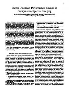
a car, then one could assume that all 4 wheels are in contact with the ground plane. If this assumption is valid, then a threshold window relative to the ground plane may be applied to remove points which are not likely to be target samples. Applying a threshold relative to the ground plane is more complicated than simply applying a threshold to the z-dimension of the point cloud data. This is due to the fact that ground topology is rarely perfectly flat. More often, the ground plane exhibits a variety of local maxima and minima. These terrain artifacts may be minimized by normalizing the ground plane, as is illustrated in Figure 1.
(a)
(b)
Fig. 1. Illustration of z -windowing. (a) Threshold on original data and (b) threshold after normalizing the ground plane.
The output of many Lidar ground plane extraction algorithms is the subset of 3D points that is believed to be representative of the ground. This set of ground points forms an irregularlygridded surface in 3D space. For the purpose of subtracting the ground plane from the point cloud data, the ground points should be interpolated using the (x, y) coordinates of the point cloud data as abscissa locations. Then the ground plane may be normalized by subtracting the interpolated ground point locations from the original point cloud data. Once in the normalized space, an upper and lower z-threshold may be applied in order to flag points that fall within the threshold boundaries. These flags should correspond to a point index in the original cloud. The original scene points corresponding to flagged indices are then retained. It is important to realize that the described flagging method does not alter the 3D geometry of the z-windowed points. Such may not be the case if points from the normalized space are retained as output. Clearly, in order for this process to be robust, accurate extraction of the ground plane is critical. While increasing the range associated with the threshold window may ease the accuracy requirements on the ground plane extraction, it may come at the expense of adding unwanted points to the remaining point cloud. Ultimately, it is important to keep in mind that the process of windowing relative to the ground plane is an optional process. The subsequent spin-image based filtering techniques will still work, albeit with higher potential for false alarms and longer run times.
2.2 Spin-image Surface Matching 2.2.1 Spin-image Fundamentals As stated earlier in Section 1, a spin-image Sp is a 2D parameter space representation of 3D shape information relative to a single oriented point p [10]. This point will be referred to as the spin-image basis point. The normal vector associated with p may be estimated via eigenvector decomposition of points within a local region relative to p and is accordingly called the spinimage basis normal np [11]. As illustrated in Figure 2, the first spin-image parameter α is defined as the perpendicular distance, relative to np , to point x. The second parameter β is the
Journal of Applied Remote Sensing, Vol. 2, 023539 (2008)
Page 3
Fig. 2. Illustration of spin-image parameters [1].
signed, parallel distance, relative to np , to point x. The mathematical representation of these parameters, also known as spin coordinates, is � � �2 β = np · (x − p) . (1) α = �x − p�2 − np · (x − p) Spin coordinates, relative to p, may be calculated for every point x in the 3D point cloud. To preserve accuracy in the spin-image generation process, spin coordinates are calculated using points from the raw point cloud. Notice that the spin coordinates (α, β) are measured in ungridded, spatial coordinates. The dimensionality reduction associated with going from 3D coordinates into the spin-image domain is described by [x, y, z] = [r, θ, z] → [r, z] ≈ [α, β] .
(2)
Assuming accurate normal estimation, the spin coordinates (α, β) should closely approximate the cylindrical coordinates (r, z), relative to point p. The cylindrical coordinate θ is ignored in the spin-image domain. A spin-image is simply a 2D histogram of the spin coordinates (α, β) associated with all points that meet three user-specified spin-image generation criteria Cs which will be described later. The first step in building a spin-image is determining which points may contribute to the spin-image Sp . This is accomplished by gridding the 3D data in spin parameter space and applying the spin-image generation criteria to the list of gridded points L{x}p . Based on the (α, β) spin coordinates associated with all of the points in L{x}p , the data is gridded according to � � � � W α 2 +β i= . (3) j= bs bs At this point, the first two spin-image generation criteria are introduced: spin support W and bin size bs . The first criterion W is used to specify the range, relative to p, over which points are allowed to contribute to a spin-image. Much like any histogram, bs specifies the range over which the spin coordinates will map to a single bin. In practice, the bin size is typically set to four times the mean sampling resolution associated with the point cloud. This is done to ensure that multiple points may map to the same bin, therein creating spin-image contrast features. These contrast features are important when performing spin-image matching. Only points from L{x}p that meet the following conditions � � � � W W j< (4) i< bs bs may contribute to Sp . The final spin-image generation criterion, spin angle Λx , is defined as � � . (5) Λx = cos−1 np · nx
Journal of Applied Remote Sensing, Vol. 2, 023539 (2008)
Page 4
Λx is a measure of the angle between np and the normal vector nx associated with point x. Λx is calculated for every point in L{x}p meeting both conditions specified in Eq. (4). Then, only the points with spin angles less than a user-specified threshold Λs are saved for the final list of � available points�L{x Cs }p (i.e., these are the only points that pass all three criteria). Once L{x Cs }p has been established, bilinear interpolation is used to reduce the error associated with the gridding process. Notice that the gridding error introduced by the floor operators in Eq. (3) is directly proportional to bs . To mitigate this error, the spin coordinates (α, β) and gridding indices (i,j) are bilinearly interpolated to calculate the contribution of a point to its surrounding grid locations. Bilinear interpolation weights are calculated according to W a = α − ibs b=β+ (6) − jbs . 2 A point’s contribution to Sp resulting from the bilinear interpolation is calculated via Sp (i, j + 1) = Sp (i, j + 1) + a(bs − b) Sp (i + 1, j + 1) = Sp (i + 1, j + 1) + (ab) Sp (i, j) = Sp (i, j) + (bs − a)(bs − b)
Sp (i + 1, j) = Sp (i + 1, j) + b(bs − a)
.
(7) � Finally, all 3D points in L{x Cs }p are binned according to Eq. (7) to form Sp . It is important to recognize that a spin-image may be generated for every point in a 3D point cloud. Figure 3 illustrates three examples of spin-images generated from a 3D-meshed rubber duckie model [10]. Each image pair, outlined in the colored boxes, is a point-specific, spin domain
Fig. 3. Example of spin-images from rubber duckie [10].
representation of the continuous (α, β) mapping of the model and the resulting gridded version of the same data, post bilinear interpolation. A spin-image representation of a 3D object may or may not be immediately recognizable, as spin-image features are directly related to radial symmetries about p. Since (α, β) coordinates are measured relative to p and np , spin-images are invariant to object orientation.
2.2.2 Library Matching Spin-image library generation is among the first steps in spin-image target detection. Spinimages are unique 2D representations of the shape information associated with 3D objects or scenes. In order to build a spin-image library, one must first have a 3D spatial model of the target. This model should be unoccluded, appropriately scaled to match the expected target
Journal of Applied Remote Sensing, Vol. 2, 023539 (2008)
Page 5
size, and of sufficient resolution to capture the 3D structure of the target. Next, the model should be spatially sampled at regular intervals to arrive at a noise-free 3D point cloud. Again, the spatial sampling interval should be at fine enough resolution to fully characterize the 3D nature of the target. Often, this spatial sampling interval will be much smaller than what may be expected in the scene data. Finally, a spin-image should be created for every point in the 3D point cloud. In practice, there is a variety of ways to generate a point cloud from a 3D object model. Most models, such as 3D Studio MaxTM and obj-based files, are facetized versions of a continuous object. While one could use the vertex information associated with these facet-based models as a point cloud, doing so may be problematic as the vertices are not typically spaced at regular intervals. For example, a single rectangular facet might be used to model the hood of a vehicle. In such a case if only the hood’s vertex coordinates were used, much of the planar information associated with the hood would be lost and therefore not contribute to the vehicle’s related spinimages. The most practical way to deal with this issue is to implement a fixed interval ray tracer from a variety of viewpoints about the model. A point should be added to the model point cloud at each intersection of a ray and continuous model geometry. The view points should be varied such that all sides of the object are sampled in order to avoid self-shadowing effects. To generate a library of spin-images, every point in a model point cloud is used as a spinimage basis point. Hence, a cloud consisting of n points results in a library of n images. While the library generation may seem relatively straightforward, the subtleties of the intelligent library generation lie in the selection of the spin-image generation criteria. The first criterion, bin size, should be sufficiently large to allow multiple points to map to a single bin. It is important to consider the contrast versus resolution tradeoff when picking the bin size. While increasing the bin size often increases the contrast across a spin-image, it also degrades the resolution in the spin-image. Considering that the same spin-image generation criteria are applied to both the model and the scene, the scene point cloud’s spacing interval should drive the bin size criterion. As such, the bin size should be set to one to two times the scene’s mean post spacing [10]. A logical choice for the second criterion, bin support, is the length of the object along its major axis. Using this construct for selecting W is ideal if one expects a scene-based target to appear with little to no external occlusion present. However, due to the fact that the largest logical size for W is being used, the corresponding spin-image is also maximized in size, thereby increasing the computational expense associated with spin-image matching. If a user expects a target to be partially hidden, then using a smaller length for W may be warranted, with the additional benefit of shorter processing times. The final spin-image generation criterion, spin angle, is useful for building self-occlusion effects into a model. The spin angle criterion should not be applied when generating scenebased spin-images, as self-occlusion is inherent in the data set. While general rules-of-thumb may be applied for setting the previous two generation criteria, picking an appropriate value for the spin angle threshold Λs is target-dependent and may be somewhat subjective. While a logical upper limit for Λs is 180◦ , using a smaller angle, such as 90◦ , may be useful for objects characterized by large-scale corner shapes.
2.2.2.1 Matching Criterion. Once the model-based library has been established, a method for matching a scene-based spin-image Ss to a spin-image from the library is needed. A criterion M for comparing the quality of a match between a given spin-image Ss and the various spinimages in the model-based library is defined as ∗ M = r(Ss∗ , Sm )·N
,
(8)
∗ where r(Ss∗ , Sm ) · N represents the correlation between the commonly populated pixels between the scene- and model-based spin-images. The correlation coefficient r, ranging between
Journal of Applied Remote Sensing, Vol. 2, 023539 (2008)
Page 6
1 and -1, measures the degree to which the function’s arguments are linearly related. If a target appears in a scene, one might expect the spin-images associated with target scene points to match closely to one or more spin-images from the model-based library. Additionally, the correlation coefficient between quality correspondence candidates should be close to 1. However, if a target is occluded in the scene, the correlation coefficient will degrade as the occlusion level increases. In order to prevent such degradation in r, only filled-bins which are common to both the scene- and model-based spin-images should be compared. Hence, the arguments of r are the scene/model spin-images where overlap, annotated by ∗ , occurs. N is the number of ∗ . The N term is important because it weights the non-zero bins that are present in Ss∗ and Sm overlapped correlation coefficient by the amount of overlap. Hence, M for a spin-image pair with only a few overlapped, highly-correlated bins may be lower than that for a spin-image pair with many overlapped, moderately-correlated bins. Finally, the correspondence for scene point s is defined as the model spin basis point s that results in the highest M score. It should be noted that the metric M is very similar to Johnson’s similarity metric S; however, a primary difference between the two is that Johnson’s metric requires an a priori estimate of the amount of target present in a scene [10]. Calculation of the M score provides an initial framework for filtering out bad scene/model correspondences. Once a model point correspondence has been established for every point in the scene, the correspondences are sorted according to their respective M scores. All correspondences with an M score that is greater than or equal to one half the maximum M score are retained [10].
2.2.2.2 Geometric Consistency. After the preliminary M-based filtering, the remaining, collective correspondence set is queried for geometric consistency. This geometric consistency filter is implemented in the spin domain and ranks point correspondences using (1) the relative distance between the correspondence’s spin-image basis points and (2) the orientations of the correspondence’s spin-image basis point normals. Recall that a correspondence consists of a scene-based spin-image and the best matched model-based spin-image, both of which are generated relative to their respective spin-image basis points. A point correspondence P (s, m) is analogous, as it defines the scene/model spin-image basis points associated with the correspondence’s respective scene/model spin-images. A point correspondence is generated for every point in the scene. The fundamental premise driving the geometric consistency filter is that the spatial relationships between point correspondences in the model domain should be similar to those in the image domain. Point correspondence pairs that are spatially inconsistent with the entire point correspondence set should be removed. Figure 4 is a conceptual illustration of correspondence pairs, with the continuous geometry for the model and scene shown for clarity. Note that the correspondences are color-coded, corresponding to match points between the scene and model. The blue and green correspondences appear to be valid, while the geometric consistency check should eliminate the red correspondence pair. Psuedocode detailing Johnson’s geometric consistency filter is provided in [10, 11]. A final set of spin-image pairs should be generated from the point correspondences that passed the geometric consistency filter. Section 2.2.3 discusses how correspondence pairs and their associated spin-images may be used to estimate which points in a Lidar point cloud correspond to target samples.
2.2.3 Recovery of 3D Target Points Although a spin-image inherently represents a reduction in the dimensionality of 3D spatial data, it does not necessarily mean that the 3D information is discarded. For example, if one were to assign an index to every point in a scene cloud, then the indices for points that contributed to a particular spin-image could be stored. Furthermore, scene points contributing to the overlapped bins between a valid correspondence pair’s spin-images could also be stored. These scene points are likely to include many target points; however, some background points may map into the
Journal of Applied Remote Sensing, Vol. 2, 023539 (2008)
Page 7
(a)
(b)
Fig. 4. Three notional correspondence points between a model (a) and a scene (b).
overlapped bins and also be included. Admittedly, this process of extracting target points is likely to have a significant number of false alarm points for low density point clouds. While the scene-points from the valid correspondences alone could be used as a target point output, it may not be reasonable to assume that every point on a target within the scene will yield a valid correspondence pair. The strength of the proposed target point extraction process is that only a single valid correspondence on or even close to (i.e., within the spin-image support criterion) a target is necessary to subsequently extract all point samples from the target. It is important to keep in mind that the accuracy of the spin-image target detection process degrades for low density clouds. Vasile and Johnson report similar numbers on the order of 200 for the required number of samples on target to ensure robust detection performance [9, 10]. For most remote sensing Lidar sensors, these sampling densities are not feasible for all but the largest of targets. As such, additional processing to mitigate false alarm locations may be warranted.
2.3 Projection onto Fixed Coordinate System The spin-image matching process described above results in a binary target label (i.e., target/not target) being assigned to each point in the Lidar data cloud. An additional step is needed in order to transform the information into a useful form relative to a secondary sensor. This transformation is achieved by projecting the geo-registered point cloud and its respective feature labels into the secondary sensor’s focal plane. In doing so, a 2D feature map is created relative to the sensor’s field of view. A framework is developed in Eqs. (9-12) to transform the 3D spatial coordinates of a Lidar point into indexed pixel coordinates associated with a secondary imaging sensor. This transformation involves two basic steps. First, one must determine the continuous location on the imager’s focal plane array (FPA) to which a scene point maps. Second, this 3D spatial location must be converted into a 2D, indexed pixel coordinate. A reference frame may be defined as a set of three orthogonal unit vectors, specifying positive directions for locating one or more points in 3D space. While the Universal Transverse Mercator coordinate system provides a common reference frame for geospatial data sets, a sensor also typically has its own reference frame S that is unique to the sensor’s pointing geometry. Obviously, two of the unit vectors will lie in the same plane as the sensor’s FPA, while the third identifies the FPA normal vector. The orientation of a sensor’s reference frame may be altered by applying a 3D rotation matrix Mxyz . A generalized definition of a sensor reference frame within a scene is given by P = Mxyz S . (9)
Journal of Applied Remote Sensing, Vol. 2, 023539 (2008)
Page 8
The columns of P are unit vectors specifying the sensor’s pointing direction and orientation. In real-world applications, the sensor’s reference frame P for a given collection geometry is often known to within the error of the Global Positioning System (GPS) and Inertial Navigation System (INS) associated with the sensor platform. Given, a sensor’s position s, orientation, and effective focal length f , one may solve for the planar intersection point q of any point g in the scene according to Pgf = t=
s + f P3 − g �s + f P3 − g�
−(P3 · g − P3 · s) P3 · Pgf
.
(10)
q = g + tPgf Pi is a unit vector specified by the i-th column of P . Pgf is defined as the unit vector pointing from scene point g to the sensor focal point. t is the scalar length of a line segment from g to its corresponding point of intersection on the FPA. Hence, t may be used to solve for the intersection point q on the FPA. This construction is illustrated in Figure 5(a).
(a)
(b)
Fig. 5. Illustration of (a) vector geometry for planar projection and (b) converting from spatial to indexed coordinates.
The second step involved in transforming the 3D spatial coordinates associated with point g is determining the FPA array bin to which the point maps. Figure 5(b) illustrates the geometry associated with this transformation. Because the sensor reference frame and all 3D point coordinates are defined relative to the global coordinate system, converting q from 3D spatial coordinates to indexed pixel coordinates for the FPA is relatively simple. Since both s and q lie in the plane defined by P1 and P2 , the linear projection of q − s onto the sensor’s respective in-plane reference frame vectors, as expressed in the equations u = (q − s) ·
P1 + ox �P1 �
v = (q − s) ·
P2 + oy �P2 �
,
(11)
yields the 2D spatial position (u, v) of q relative to s, as measured by the sensor’s reference frame. Note that ox and oy specify the center of the FPA. Finally, the continuous, spatial coordinates (u, v) may be converted to indexed coordinates (i, j) specific to the FPA according to � � � � u v i= j= . (12) bx by
Journal of Applied Remote Sensing, Vol. 2, 023539 (2008)
Page 9
The terms bx and by represent pixel pitch, and � � is the floor operator. It should be noted that this framework does not account for geometric distortion in the sensor’s optics, nor does it account for distortion due to scanning mechanisms or spectral artifacts. While the above derivation applies directly to mapping 3D points onto a 2D FPA used in frame imaging systems, a similar approach could be used to model linear arrays used in pushbroom scanning systems. In such a case, the sensor’s origin s and reference frame P would need to be updated as the sensor’s field of view (FOV) traverses the sensor ground track.
2.4 Pixel Purity Map Pixel purity refers to the fractional percentage of a pixel that is filled by a target object. To create the purity map, all target samples are projected into the imaging FPA according to Eqs. (9-12). Since subpixel information is to be captured in the resulting pixel purity map, the points need be projected onto a fine-scale grid, which may be accomplished by subdividing the pixel pitch in Eq. (12). Finally, pixel purity for a given pixel is calculated as 2
n
M=
i=1
mi
n2
,
(13)
where mi is the binary fill value for the i-th subgrid location within a given pixel and n is the number of locations in the subgrid along a single dimension. Bright regions in the pixel purity map represent pixels with high target fill factors.
3 RESULTS 3.1 Synthetic Data Synthetic point clouds were generated using the Digital Imaging and Remote Sensing Image Generation (DIRSIG) simulation tool [12]. After simulating the geometry of an area on the Rochester Institute of Technology campus referred to as Microscene, two different point clouds were created. A noise-free point cloud, shown in Figure 6(b), is used to demonstrate the performance of spin-image based matching for ideal data with a mean post spacing of 0.2 m. As a comparison point, a noisy data point cloud of the same area was generated to illustrate the impact of several different system error sources, to include pointing error, platform location uncertainty, and range quantization. The numeric labels on the ground truth image in Figure 6(a) correspond to the following ground truth: 1. 2. 3. 4. 5.
Gray Humvee Calibration panel Gray SUV† Gray shed Red sedan
6. 7. 8. 9.
Red SUV† Gray SUV† hidden under tree Gray SUV† inclined on berm Gray Humvee inclined on berm
Legend: † = 3D target shape A library of spin-images was constructed based on a CAD model of an SUV using the following spin-image generation criteria: • Spin support = 4.0 m • Bin size = 0.2 m • Spin angle = 20◦
Journal of Applied Remote Sensing, Vol. 2, 023539 (2008)
Page 10
(a)
(b)
Fig. 6. Microscene data. (a) Reference true color simulated image used for ground truth and (b) oblique view of ideal Lidar point cloud false colored by height.
After z-windowing based on an extracted ground plane, the spin-image filtering of the Microscene point clouds produced a number of correspondence pairs and subsequent extracted target points. Finally, the extracted target points were projected into the same reference frame as the image shown in Figure 6(a). The result of the projection is shown in the pixel purity maps in Figure 7.
(a) (b) Fig. 7. Pixel purity maps derived from Microscene Lidar data. (a) Ideal and (b) Noisy.
It is important to recognize that the result of the spin-image surface matching algorithm is largely dependent upon the user-selected spin-image generation criteria. The brightest features in the pixel purity map in Figure 7(a) correspond to manmade features. The implemented spin-
Journal of Applied Remote Sensing, Vol. 2, 023539 (2008)
Page 11
image matching routine detected all objects with planar surface features, despite the fact that the library was based on the SUV model only. Despite the fact that the ideal and noisy point clouds have roughly equivalent mean post spacings, the spin-image filtering performance degrades considerably once noise is introduced, as illustrated in Figure 7(b). This is partially due to the implemented target point extraction process, as described in Section 2.2.3. However, the most significant impact on spin-image matching results from range quantization. Range quantization forces points within the same range bin to align themselves in a plane that is perpendicular to the Lidar illumination (i.e., range) direction. As a result, much of the local shape information may be lost, producing poor estimates of local surface normals. Recall that the basis vectors in the spin-image space are derived from such normals. Hence, range quantization effectively rotates the basis functions for scene-based spin-images, ultimately limiting the matching performance.
3.2 Real Data In the fall of 2006, the Leica Corporation overflew the RIT campus, to include the Microscene I area, with an ALS 50 instrument. The ALS 50 is a line scanned topographic Lidar system, operating on a laser line center of 1.064 µm with a pulse width of 0.5 ns. At the time of the collect, the microscene area contained one vehicle inclined on the archery berm. The resolution of the resulting processed point cloud was approximately 0.4 m in the direction of flight and 0.25 m along the scan direction. Figure 8 shows a screen capture of the Leica data set for Microscene I and an image of the target vehicle within the scene. The visualization of the
(a)
(b)
Fig. 8. (a) Range image of Leica point cloud (b) Image of pickup truck within Microscene I. R point cloud was produced using the Merrick Advanced Remote Sensing (MARS � ) software utility [13]. Application of the described spin-image target detection techniques on the Leica data proved to be an interesting challenge. Not only did the collect provide data with true noise artifacts, but also the sampling density on the pickup was extremely limited. Inspection of the data cloud revealed that approximately 30 point samples actually fell on the truck; hence, estimation of accurate surface normals would be difficult at best. Leica applied proprietary preprocessing techniques to their raw point clouds in order to eliminate false returns and geo-register the points. Furthermore, in delivering the processed clouds, Leica also supplied extracted, noninterpolated ground plane points for the clouds. These ground points were used to apply a z-window to the data prior to the spin-image filtering. Next, the remaining z-windowed points were filtered based on the following spin-image generation criteria:
• Spin support = 5.0 m • Bin size = 0.3 m
Journal of Applied Remote Sensing, Vol. 2, 023539 (2008)
Page 12
• Spin angle = 30◦ A notional imaging sensor was created for the purpose of projecting the extracted target points onto an FPA. The hypothetical sensor was pointed at the scene center and designed to have a GIFOV of 1.0 m when oriented at Nadir. The pixel purity map derived from the Leica data is presented in Figure 9. Similar to the previous noisy, simulated data set, the result in
Fig. 9. Pixel purity map for Leica point cloud and notional imaging sensor (vehicle outlined in red).
Figure 9 has a significant number of false alarm locations. However, it is interesting to note that all of the samples from the truck resulted in valid correspondence points and the second highest ranked correspondence for the entire scene was a true scene correspondence located on the hood of the pickup truck. Given the number of correspondences in the point cloud, the high scoring correspondence on the truck is not likely to be coincidental. While these output correspondences could be thresholded according to their respective geometric consistency scores, a logical method for determining an appropriate threshold value proved to be elusive. Hence, all correspondences were retained in hope of suppressing false alarms via one or more secondary processes.
4 SUMMARY The Johnson spin-image surface matching algorithm was applied to several low density Lidar point clouds. Several different factors result in decreased matching performance. (1) Low density clouds may not have sufficient sampling resolutions to allow for accurate statistics when constructing spin-image histograms. (2) Noise artifacts, such as point location error and range quantization, can result in a significant rotation of the basis functions for scene-based spinimages. While bilinear interpolation is used as an error mitigation method, its effectiveness is inversely related to a point’s α value (i.e., radial distance relative to spin-image basis normal) within the spin-space. That said, the spin-image techniques may prove to be effective as a preprocessing (i.e., cueing) step in exchange for a significantly reduced search space for applications that can tolerate a high number of false alarms. Finally, a framework for projecting a 3D point into an arbitrary, gridded viewing frame was presented. Such a projection may used as a target detection map or as a means to fuse Lidar point clouds with traditional imagery. Future work in this area is focused on fusing the Lidar-based target nomination maps with spectral imaging data to improve target detection in the presence of clutter.
Journal of Applied Remote Sensing, Vol. 2, 023539 (2008)
Page 13
Acknowledgments The authors would like to thank the Leica Corporation for providing Lidar data of the RIT campus.
References [1] Y.-T. Zhou and D. Sapounas, “IR/ladar automatic object recognition system,” Automatic Target Recognition VII 3069(1), 119–128, SPIE (1997). doi:10.1117/12.277096. [2] M. R. Wellfare and K. Norris-Zachery, “Characterization of articulated vehicles using ladar seekers,” Laser Radar Technology and Applications II 3065(1), 244–254, SPIE (1997). doi:10.1117/12.281016. [3] F. A. Sadjadi, “Application of genetic algorithm for automatic recognition of partially occluded objects,” Automatic Object Recognition IV 2234(1), 428–434, SPIE (1994). doi:10.1117/12.181040. [4] e. Snorrason, M., “Automatic target recognition in laser radar imagery,” in Acoustics, Speech, and Signal Processing, International Conference on, 4, 2471–2474, ICASSP (1995). doi:10.1109/ICASSP.1995.480049. [5] Q. Zheng, S. Der, and H. Mahmoud, “Model-based target recognition in pulsed ladar imagery,” Image Processing, IEEE Transactions on 10, 565–572 (2001). doi:10.1109/83.913591. [6] F. Cobzas and H. Zhang, “Planar Patch Extraction with Noisy Depth Data,” Third Intl. Conf. on 3-D Digital Imaging and Modeling , pp. 240–245 (2001). doi:10.1109/IM.2001.924444. [7] G. Stein, F.; Medioni, “Structural indexing: efficient 3-D object recognition,” Pattern Analysis and Machine Intelligence, IEEE Transactions on 14, 125–145 (1992). doi:10.1109/34.121785. [8] O. Carmichael and D. Huber, “Large Data Sets and Confusing Scenes in 3-D Surface Matching and Recognition,” in Proc. of Second Intl. Conf. on 3-D Imaging and Modeling, pp. 358–367, (Ottawa, CA) (1999). doi:10.1109/IM.1999.805366. [9] A. N. Vasile and R. Marino, “Pose-independent automatic target detection and recognition using 3D LADAR data,” Automatic Target Recognition XIV 5426(1), 67–83, SPIE (2004). doi:10.1117/12.546761. [10] A. Johnson, Spin-images: A Representation for 3-D Surface Matching. PhD dissertation, Carnegie Mellon University, 5000 Forbes Avenue, Pittsburgh, PA (1997). [11] M. Foster, Using Lidar to Geometrically-constrain Signature Spaces for Physics-based Target Detection. PhD dissertation, Rochester Institute of Technology, 54 Lomb Memorial Drive, Rochester, NY (2007). [12] S. Brown, DIRSIG User’s Manual, Release 4. Chester F. Carlson Center for Imaging Science, Rochester Institute of Technology, 54 Lomb Memorial Drive, Rochester, NY 14623-5604 (2006). http://dirsig.cis.rit.edu/doc/manual/manual.html. [13] Merrick and Company. http://www.merrick.com/servicelines/gis/mars.aspx, Merrick and Company website, June 2007.
Author Biographies Michael S. Foster received his BS degree in physics from the United States Air Force Academy in 1999 and his PhD degree in imaging science from the Rochester Institute of Technology in 2007 as part of the Air Force Institute of Technology’s Civilian Institution program. John R. Schott is the head of the Digital Imaging and Remote Sensing group within the Chester F. Carlson Center for Imaging Science at RIT. He received his BS degree in physics/sociology
Journal of Applied Remote Sensing, Vol. 2, 023539 (2008)
Page 14
from the Canisius College in 1973 and his MS and PhD degrees in Environmental Engineering and Environmental Science from the Syracuse University in 1978 and 1980, respectively. He is the author of more than 50 journal papers and has written two books on remote sensing. He is a member of SPIE. David W. Messinger is a faculty member within the Chester F. Carlson Center for Imaging Science at RIT. He received his BS degree in physics from the Clarkson University in 1991 and his PhD degree in physics from the Rensselaer Polytechnic Institute in 1998. He is a member of SPIE.
DISCLAIMER The views expressed in this article are those of the authors and do not reflect the official policy or position of the United States Air Force, Department of Defense, or the U.S. Government.
Journal of Applied Remote Sensing, Vol. 2, 023539 (2008)
Page 15