Using the MaxD Target Detection (MaxDTD) Algorithm in ENVI with AVIRIS Data ∗ Emmett J. Ientilucci Chester F. Carlson Center for Imaging Science Rochester Institute of Technology
[email protected] January 12, 2004
Abstract This report accompanies the MaxD target detection algorithm implemented in the ENVI environment. The intent of the report is to describe the results obtained by using a provided AVIRIS test data set. Topics addressed include basic results on implementing the test data, how the test data set was processed and calibrated, and how the sensor response was applied. A brief analysis of results beyond the typical algorithm run is also discussed.
1
Introduction
This document describes various aspects of using the MaxD target detection algorithm with a test AVIRIS data set. The report is divided into (5) sections. Section 2 explains what (test) files are required to run the algorithm and how to achieve a result. Section 3 describes details of the data including dimensions, calibration procedures used, units issues, and how to incorporate a bad bands list and sensor response. Section 4 examines some of the intermediate results during processing of the algorithm. Additionally, some analysis is performed on the resultant data. Additional information on the MaxD algorithm can be found in [1, 2]. Performance analysis on how the MaxD algorithm performs relative to other basis-vector selection techniques can be found in [3].
2
Using the Algorithm with Test Data
A test data set has been provided so as to check one’s installation or configuration of the target detection algorithm. This section uses the test data with the default algorithm settings and generates a result. The following files (see Table 1) are required to complete a single run of the algorithm. These include the spectral reflectance of a target, atmospheric look-up-table (LUT), and a (hyperspectral) image. The algorithm and test data set are run as follows: • After ENVI starts up, select the MaxDTD button the on the tool bar and select Target Basis Vectors. • Select the target spectrum (red_basketball_ct.sli), AVIRIS look-up-table (aviris_roch_448.lut), and calibrated imagery (aviris_roch.img) as shown in Figure 1. We will omit the sensor noise in this example. ∗ This
file has version number v1.0, last revised on 1/12/04
1
Table 1: Names and descriptions of files included in the test data set. Filename Description red_basketball_ct.sli Target spectral reflectance in ENVI spectral library format [µm] red_basketball_ct.sli.hdr Target spectral reflectance ENVI header aviris_roch_448.lut MODTRAN generated look-up-table (LUT) based on AVIRIS image [W cm−2 sr µm] aviris_roch.img AVIRIS image [W cm−2 sr µm] 100 samples × 100 lines × 200 bands aviris_roch.img.hdr AVIRIS image ENVI header
Figure 1: Target basis-vector dialog box. • Under Options, use the default settings for the number of vectors created with MaxD and FSR. • After the Process button has been selected, the routine creates a set of target basis-vectors in ENVI’s spectral library format. The new target basis-vector spectral library has the name red_basketball_ct.sli_basis.sli. • We now apply the new target basis-vectors to the image. Select the MaxDTD button once again on the tool bar and select Background Basis Vectors. • Select the same image as before (aviris_roch.img) and new target basisvectors (red_basketball_ct.sli_basis.sli) as shown in Figure 2. • Under Options, use the default settings for the number of vectors created with MaxD and FSR. • After the Process button has been selected, the algorithm should create a probability map like that shown in Figure 3.
Figure 2: Background basis-vector dialog box.
2
(a)
(b)
Figure 3: Probability maps, with (a) square root stretch and (b) linear threshold, generated with the MaxDTD tool. 1200 1000
Gain Factor
800 600 400 200 0 0
50
100
150
200
250
Band
(a)
(b)
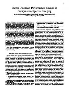
Figure 4: (a) AVIRIS 100 × 100 image. Bands 9, 19, and 29 are displayed. Two regions, containing interesting targets, are circled. The region on the left contains a red basketball court while the region on the right contains a red tennis court. Higher resolution imagery of these targets can be seen in Figure 5. (b) AVIRIS image multiplication factors.
3
Processing the Data
This section describes details of the AVIRIS data and how the test files were created. The software used for analysis and running of the algorithm was ENVI version 4.0. The sample AVIRIS image [see Figure 4(a)] is of Rochester, NY, and contains 100 samples × 100 lines × 200 bands (0.4004 µm to 2.498 µm). In its original form, the file contained 224 bands (0.3709 µm to 2.507 µm), however, the first 3 bands, as well as the last band, were truncated (using Basic Tools/Resize Data in ENVI) to match the dimensions and band centers of the MODTRAN generated look-up-table. The original data were in units of G · [µW cm−2 sr nm], where G is a multiplication factor used to store the image radiance values as 16-bit signed integers (IEEE byte order). The data were then converted to radiance [µW cm−2 sr nm] by dividing by the AVIRIS spectral gain factor [see Figure 4(b)].
3
3.1
AVIRIS Calibration Procedure Using ENVI
Here we multiplied each band by the appropriate multiplication factor to yield an image in radiance units [µW cm−2 sr nm]. The gains were made part of the image header file and applied thereafter. Prior to including the gains in the header, one needs to have an ASCII file containing a single column of gains prepared. For this AVIRIS image, a file containing 220 entries was prepared. Bands 4-160 (the first 157 lines in the file) had a gain of 0.002 (1/500) while bands 161-223 (the last 63 lines of the file) had a gain of 0.001 (1/1000). The procedure was as follows: • Open the image in ENVI. • Edit the image header. File/Edit ENVI Header. • Under Edit Attributes, select Gains. • In the Gains dialog box select Import ASCII, and select the prepared gain file created earlier. • Apply the column of gains and save the header file. • Select Basic Tools/Preprocessing/General Purpose Utilities/Apply Gain and Offset. Select the image file and apply the gains. Units are now [µW cm−2 sr nm].
3.2
Convert AVIRIS Image to LUT Units and Apply Sensor FWHM
At this point the AVIRIS image units are [µW cm−2 sr nm]. The MODTRAN generated look-up-table (LUT) units are [W cm−2 sr µm]. The AVIRIS data can be converted to LUT compatible units by using Band Math in ENVI. Multiplying each band by 0.001 will convert the AVIRIS data to LUT units. • In ENVI select Basic Tools/Band Math. Type the equation b1 * 0.001. • Map the variable “b1” to the “AVIRIS” input file. Save result. Additionally, we have to change the wavelength representation from [nm] to [µm]. Finally we apply the sensor response, in microns, to the image. The last two steps are accomplished by editing the image header and reading in an ASCII file containing 2 columns. Column one being wavelengths [µm] and column two being sensor FWHM [µm]. • Edit the image header. File/Edit ENVI Header. • Under Edit Attributes, select Wavelengths. • In the Wavelengths dialog box select Import ASCII, and select the prepared sensor response file. • Assign the columns to the appropriate variables. • In the Edit Wavelength Values dialog box, be sure to select Micormeters for the wavelength units. Select OK and update the header.
4
(a)
(b)
Figure 5: High resolution aerial imagery of a (a) red basketball court and (b) green tennis court playing surface surrounded by a (similar) red region. An AVIRIS pixel is drawn over each court to indicates its size relative to the hi-res imagery.
3.3
Specifying Bad Bands List Using ENVI
During processing we would like to omit bands that do not contain useful information due to CO2 or H2 O absorption, poor SNR in a band, etc. ENVI has the ability to keep track of these “bad bands” through manipulation of the image header. For this 220 band test data set, (4) regions (between bands 4 and 223) have been marked as bad. The bad bands are: 4 (0.400µm), 107-121 (1.355µm-1.495µm), 152-181 (1.803µm2.081µm), and 202-223 (2.290µm-2.498µm). This leaves a total of 152 valid bands. The procedure for defining bad bands is as follows: • Edit the image header. File/Edit ENVI Header. • Under Edit Attributes, select Bad Bands List. • Select the appropriate valid bands, click OK and update the header.
3.4
Creating a Spectral Library Target File Using ENVI
There are (2) keys targets in the AVIRIS test imagery, as indicated previously in Figure 4(a). Both of these targets have red court playing surfaces (as indicated in Figure 5). A ground measurement collections team visited both sites and provided a reflectance spectrum of the surface as measured by a hand held spectrometer (see Figure 6). These data need to be in ENVI’s spectral library format in order to function properly with the MaxDTD tool. The procedure for creating the spectral library used in this report is as follows: • In ENVI, select Spectral/Spectral Libraries/Spectral Library Builder. • In the Spectral Library Builder dialog box select ASCII File. • Assuming the data format is ASCII, select the appropriate reflectance file to read in. Be sure the units are microns. • This time in the Spectral Library Builder dialog box select Import/from ASCII file. • Select the spectral reflectance file to import and click OK. • Save the spectrum by selecting File/Save Spectra As/Spectral Library. 5
0.4 0.35
Reflectance
0.3 0.25 0.2 0.15 0.1 0.05 0 0
0.5
1
1.5
2
2.5
3
Wavelength [um]
Figure 6: Ground measured reflectance spectrum of a red basketball playing surface.
Figure 7: Plot of 15 target basis vectors with the red target pixel from the AVIRIS image over-plotted (red, heavy line).
4
Analysis of Results
This section takes another look at the algorithm results and intermediate steps involved in using the provided test data set.
4.1
Target Basis-Vectors
Here we compare the target basis-vectors created with the target pixel of interest (red basketball court). A plot that overlays 15 or so target basis vectors with the pixel containing the red basketball court can be seen in Figure 7. We can see that the basis vectors line up reasonable well with the target pixel. Any mismatch can be attributed to the target pixel being mixed (i.e., not a fully resolved red pixel), the measured reflectance spectrum not being a true representation of the red playing surface, or the parameters used to model the atmosphere in the image being slightly off.
6
Figure 8: GLR probability map. The x-axis is pixel number while the y-axis is proportional to a probability of detection.
4.2
GLR Probability Plot and Map
This section talks about the probability plot and map that is generated during run time. An example of the probability plot associated with the results of Figure 3, can be seen in Figure 8. Here we see a few distinctive “spikes” that correspond to high detection probabilities associated with the red-court pixels. Further analysis of the probability map (see Figure 9) shows that, given the appropriate threshold, the first 3 pixels in the detection are truly from the desired target. The fourth highest probability pixel is a false alarm. Better results (fewer false alarms) may be achieved by adjusting the number of target and background basis vectors used in the analysis.
5
Concluding Remarks
This report gives a basic overview of how to use the MaxD algorithm, as well as expected results, using the provided sample AVIRIS data set. One should be able to generate similar results given that the algorithm has been installed correctly. Additionally, an overview of how the data were processed before it was implemented in the algorithm was discussed. Finally, a brief analysis was given on algorithm results. It is believed that better results, other than stated in this report, may be obtained by varying the number of basis vectors used. However, at this time, we do not address the issue of optimal basis vectors. The intent of this report was to provided a working test data set with a brief description of results.
7
Figure 9: GLR target detection probability map. Implementing a threshold illustrates that the first 3 pixels are of the basketball court.
References [1] K. Lee. A subpixel scale target detection algorithm for hyperspectral imagery, PhD dissertation, Rochester Institute of Technology, 54 Lomb Memorial Drive, Rochester, NY, 2003. [2] J.R. Schott, K. Lee, R. Raqueno, G. Hoffmann, and G. Healey. A subpixel target detection technique based on the invariance approach. To be published, 2004. [3] P. Bajorski, E.J. Ientilucci, J.R. Schott, Comparison of basis-vector selection methods for target and background subspace as applied to subpixel target detection. To be published in Proc. SPIE, Algorithms and Technologies for Multispectral, Hyperspectral, and Ultraspectral Imagery X, Orlando, FL, April 2004.
8