Stabilized Least Squares Finite Element Method for 2D and ... - WSEAS

WSEAS TRANSACTIONS on APPLIED and THEORETICAL MECHANICS

V. D. Pereira, J. B. C. Silva, L. F. M. Moura, E. C. Romão

Stabilized Least Squares Finite Element Method for 2D and 3D ConvectionDiffusion

V. D. PEREIRA1, J. B. C. SILVA2, L. F. M. MOURA1 and E. C. ROMÃO3 1

Thermal and Fluids Engineering Department, Mechanical Engineering Faculty, State University of Campinas, Campinas/SP, Brazil. 2UNESP – Ilha Solteira, School of Engineering of Ilha Solteira, Mechanical Engineering Department, Av. Brasil 56,

15385-000, Ilha Solteira – SP, Brazil. 3Department of Basic and Environmental Sciences, EEL-USP, University of São Paulo, Lorena/SP, Brazil * Correspondence: E. C. Romão. E-mail: [email protected]

Abstract - In this study, a computational code has been developed based into Finite Elements Method in the version of LSFEM (Least Squares Finite Element Method). The numeric development of this method has as a main advantage, the obtaining of an always symmetrical and defined positive algebraic system, independently of the considered partial-differential equation system. The computational code was applied in the solution of two-dimensional and three-dimensional convection-diffusion problems, through domain discretization of structured meshes of quadratic elements. Obtained numerical results showed a good concordance with available results, showing the developed model validity. Keywords - Finite Element Method, Least Squares, Convection, Diffusion, Peclet number, Conjugate Gradient Method.

Least Squares Finite Element Method (LSFEM) is a method that has been investigated for fluid flow simulation, and according to Jiang, for example, does not require utilization of “upwind” techniques. Upwind techniques have difficult implementation in multidimensional problems. Although p refinement version is a way of reducing some of LSFEM defects, it was opted by adopting h refinement of mesh with quadratic elements with lagrangian functions, in order to verify the result quality of these elements at Least Squares version, because they are elements that have already been used by the research group in other applications of the Finite Element Method. [5] showed a formulation of Least Squares Finite Element Method with p refinement for Convection-Diffusion equation solution. The second order differential equation, describing the Convection-Diffusion problem is transformed in a equivalent set of first order differential equations, in which the Least Squares formulation is constructed using the same order approximation to each dependent variable. The functions of hierarchical approximation and the nodal variable operator are established by the construction of function of unidimensional hierarchical approximation of order pξ and pη in directions ξ and η. Bidimensional polynomials

1 Introduction Fluid flow calculations are important to both man and nature. Such flows are mathematically modeled by Navier-Stokes equations, which are nonlinear partialdifferential equations and, therefore, of difficult analytical solution, except in very much simplified cases. In view of nonlinearities and geometric complications found in real problems, solutions of the Navier-Stokes equatio, in their complete form, are only possible by means of numerical methods. The Finite Element Method has its mathematical basis on the weighted residual methods (WRM), which gives origin to its several formulations: Galerkin-Bubnov, Petrov-Galerkin, Collocation, Subdomain and Least Squares. These formulations result from the chice of the weight function in the internal product of this by residue in the variational or integral formulation of the method. The current literature on the Finite Element Method is broad, highlighted on [1-4] text-books. [4] presents in details a formulation of the Least Squares Finite Element Method (LSFEM – Least Squares Finite Element Method) for computational fluids dynamics and electromagnetism.

E-ISSN: 2224-3429

45

Volume 9, 2014


frequently by some p elements, being the basic for a higher order approximation. [10] made applications with Least Squares Finite Elements method combined with spectral / hp methods for numerical problem solutions of viscous fluid flow. The study shows an hp spectral algorithm formulation, validation and application for a numerical solution of bi and tridimensional Navier-Stokes equations for incompressible stationary flows and low-speed compressible flow. The Navier-Stokes equations are expressed as a set of equations of first order through introduction of vorticity and velocity gradients as independent additional variables. Expansions in high order element are used to build the discreet model. The discreet model is obtained by Newton’s method linearization, resulting a linear system of equation with a symmetrical and defined positive coefficient matrix, which is solved by preconditioned conjugate gradient method. Functional convergence of Least Squares method and rule error are verified by means of solutions of stationary bidimensional Poisson’s equation and incompressible Navier-Stokes equations. Numerical results for permanent flow on a circular cylinder, tridimensional flow in a cubical cavity, and a compressible flow with natural convection in a cavity are presented to demonstrate predictive capacity and strength of the proposed formulation. Finally, numerical results for flow in a lid-driven cavity are presented to demonstrate the effectiveness of iterative procedure in the Least Squares Finite Elements method. In [11], the Navier-Stokes equations for flowing in an airplane are reformulated as a system of first order depending on tension and streamfunction. Solutions of this system are obtained by LSFEM. A characteristic of this approach is that, after system linearization, the algebraic problem will be symmetrical and defined positive in each Newton’s iteration. Care as for incompressibility treatment is necessary to guarantee good results.

are constructed by the product of unidimensional polynomials. Numerical results were showed and compared with numerical and analytical solutions in a bidimensional test problem for demonstrating the precision of convergence characteristics in this formulation. [6] presented a formulation of Finite Element with p refinement for a nonlinear problem of incompressible, bidimensional and permanent fluid flow. The Navier-Stokes equations were modeled as equations of first order, involving viscosity and shear stresses as auxiliary variables. Both auxiliary and primitive variables were interpolated using C0 continuity and of equal order. Least Squares error functional is constructed using a system of partial-differential equations of first order, coupled without linearization, approximations and other suppositions. Numerical examples were showed to demonstrate convergence and precision characteristic of this method. [7] have utilized Least Squares method for approximated solution for Stokes’s equation which results in a pression-velocity-vorticity system of first order. Among the most attractive characteristics of applied methods is that they result in a symmetrical and definedpositive system of algebraic equations. [8] showed a Least Squares Finite Elements formulation with p refinement for a bidimensional nonpermanent fluid flow described by Navier-Stokes equations from where space and time effects are coupled. Element proprieties are derived using p refinement, approximation functions in space and time, by minimizing the functional formed by integration of sum of square errors. A time step procedure is developed in the way solution stops at the current time step and provides initial conditions for the next step. Coupled equations in space-time of p-version approximation provide ability for truncation error that, in turn, allows very large steps of time. What is literally required by the hundreds of time steps in conventional uncoupled procedures can be performed at a single time step, using the current space-time of coupled approximation. Results were compared with analytical solutions and those reported by the literature. The showed formulation is ideal for adaptable space-time procedures. Element error functional values provide a mechanism for h, p or h-p refinement. [9] show an implementation of a p tridimensional version for structural solid problems with almost arbitrarily curved surfaces. Applying the method of function mixture, complex structures can be modeled

E-ISSN: 2224-3429


2 Mathematical Model for Tridimensional Convective-Diffusive Problems Initially consider the Energy equation in the form [5],

 ∂ 2T ∂ 2T ∂ 2T   ∂T ∂T ∂T   = k  2 + 2 + 2  +v +w ∂y ∂z  ∂y ∂y   ∂x  ∂x

ρc p  u

(1) where T is the temperature field; u, v and w are the components of the velocity field; ρ is the density; c p

46

Volume 9, 2014



is the specific heat at constant pressure; k is the thermal conductivity.

where E1 , E2 , E3 and E4 are the errors and the index h represents the element size. The formulation of Least Squares Finite Elements can be seen as a variational approximation, in the sense that a functional minimizing is searched. In this way, it is defined the following functional for an element

The equation (1) can be rewritten, as

ρ uc p

∂T ∂T + ρ vc p + ∂x ∂y

∂T ∂q x ∂q y ∂qw + + + = 0 (2) ∂z ∂x ∂y ∂zˆ = Ie F (T h , qxh , q yh , qzh ) d Ω (10) The components of heat flux are given by the Ω Fourier´s law: ∂T In the case of a single differential equation written in a (3) qx + k =0 ∂x compact form as AT = f ; the function inside the ∂T integral is F = E 2 , where AT h − f = E . For a system (4) qy + k =0 ∂y of N differential equations, F is taken as a sum of N ∂T (5) qz + k =0 squared errors, that is, F = Ei2 , so the global ∂z i =1

ρ wc p

∫

∑

functional in the whole domain will be given by the expression

3 Least Squares Finite Elements Method Equation (2) to (5) constitutes a system of first order h h h h partial differential equations. With T , qx , q y e qz as

I=

Finite Elements approximations for the true solutions T , qx , q y , qz , it is possible to define the

(

N

(12)

i =1 Ω e

If the vector of unknowns is defined by the expression:

∂T h ∂T h ∂T h ∂T h +u +v +w − ∂t ∂x ∂y ∂z

{δ }

T

T T T T = {T } , {qx } , {q y } , {qz }   

(13)

(6) the minimization of functional in Equation (12) requires that

∂I e (7)= ∂ {δ }

q yh −

∂T h = E3 ∂y

(8)

qzh −

∂T h = E4 ∂z

(9)

E-ISSN: 2224-3429

(11)

I e = ∑ ∫ Ei2 dΩ

following residues or errors for approximated solutions within an element, so equations (2) to (5) are rewritten for the approximant variables in dimensionless form, including a transient term, as:

∂T h qxh − = E2 ∂x

Ie

e =1

)

h 1  ∂qxh ∂q y ∂qzh  −  + + E1 = Pe  ∂x ∂y ∂z 

∑ NE

∑∫ 3

i =1

∂Ei = Ei d Ω 0 Ωe ∂ {δ }

(14)

Equation (12) is the functional form when each residue is individually considered. In the context of Finite Elements, variables are interpolated in the element by expressions:

T h = [ N ] {T }

47

(15)

Volume 9, 2014



qxh = [ N ] {qx }

(16)

q yh = [ N ] {q y }

(17)

qzh = [ N ] {qz }

(18)

1  0 A0 =  0  0

[ N ] is the matrix of interpolation functions and {T }, {q x } , {q y } and {q z } are the nodal variables for T h , qxh , q yh and qzh , respectively.

 v  A2 =  0  −1  0  w  A3 =  0 0   −1

Equations (6) to (9) constitute a nonlinear problem of initial and boundary values, which after time discretization, following [4], can be written as:

+ θ  A (ϕ )  ∆t *

n +1

= f *

(19)

where n  ∂ϕ  ∂ϕ ∂ϕ *  A (ϕ )  =  A1 ∂x + A2 ∂y + A3 ∂z + A4ϕ   

f = *

ϕ

n

n

− (1 − θ )  A (ϕ )  + f ∆t *

n

(20) (21)

where θ is a parameter that represents the time discretization scheme, since an explicit method until a totally implicit method and n indicates time step. Following [2]:

θ

0  0 A4 =  0  0 

0, backwards differencescheme (or Euler scheme)  = O(∆t ) conditionally stable, order of precision 1 2  2 , Crank's scheme-Nicolson (stable); O((∆t ) ) 2 2  3 , Galerkin's method (stable); O((∆t ) ) 1, forward difference scheme (stable); O( ∆t )

= f

T

∂( ) ∂( ) ∂( ) + A2 + A3 + ∂x ∂y ∂z

A  +  0 + A4   ∆t 

0

0 0 0 0

0 1 0 0

 0 0  0 0 0 0  0 0 

(25)

−1  0 Pe  0 0 0 0  0 0  −1  0 Pe   0 0  0 0   0 0  0 0  0 0 1 0  0 1 

(26)

(27)

(28)

A0 n ϕ − (1 − θ ) A* (ϕ n ) ∆t

(29)

= R A(ϕ e ) − f

(30)

For applying the Least Squares Finite Element method, it is defined a functional at an element as follows: (23)

= Ie

∫

RT ⋅ Rd Ω

Ωe

with the coeffients Ai defined as follow:

E-ISSN: 2224-3429

0 0

(24)

If φe is an approximated solution for φ inside an element, it is possible to get an alternative formulation by defining a residual vector R from Eq. (21) as

where ϕ = T , qx , q y , qz  are the variables and A is a differential operator defined as

) = A1

0

0  0 0  0 

The source term in Equation (22) is defined as

Equation (19) can be rewritten in a compact form as A (ϕ ) − f = 0 (22)

A(

0 0 0 0

−1   u Pe  A1 =  −1 0 0 0  0 0

where

ϕ n +1

0 0 0 0

48

(31)

Volume 9, 2014



∫

Similar to the functional minimizing defined in Eq. (12), by considering the Equation (31) we also have

δ Ie = 0;

Ωe

rewritten in the form:

∫

Ωe

δ R ⋅ Rd Ω =0 T

Ωe

(33)

δ R = A (δϕ )

[ N ]{δΦ}

K=

(35)

∑

K

(36)

= F e

(37)

ϕ = e

∑ j =1

;

Fe

e =1

(42)

∫ ∫

Ωe

Ωe

AT ( N ) A( N )d Ω A ( N ) { f }d Ω

;

T

(43)

(22), A( N ) can be defined as a matrix:

 a11 a12 a a A( N ) =  21 22  a31 0   a41 0

a13 0 a33 0

a14  0  0  a44 

(44)

with coefficients (38)

Using Equations (36) and (37), Equation (35) can be rewritten as

E-ISSN: 2224-3429

∑

and by substitution of Ao , A1 , A2 , A3 , A4 in the Equation

and the nodal vector of unknowns. If an element is defined by Nn nodal points with ndof degrees of freedom per node, Equation (36) can also be rewritten as:

Φ1  Φ   2  Nj     Φ ndof   j

F=

e

in which

[ N ] and {Φ} are the matrix of interpolation functions

Nn

(40)

Nelem

Nelem

= Ke

= δϕ e

AT ( N ) { f }d Ω

where K is the global matrix of the coefficients, Φ is the vector of unknowns and F is the vector source-terms. The matrix K and the vector of source-terms are obtained from the assembling for all elements, that is,

(34)

e =1

and therefore, the variation of ϕ e is:

Ωe

(41)

The vector of unknowns is interpolated in the form:

[ N ]{Φ}

∫

K Φ =F

Substituting Equations (30) and (34) into Eq. (33), it is obtained T e e e ∫Ωe A (δϕ )  A (ϕ ) − f d Ω =0

AT ( N ) A = ( N )d Ω {Φ}

Adding collectively the contribution of all elements, the following system of algebraic equations is obtained

in which the first variation of residue is defined from the Equation (30) as

= ϕe

(39)

For δΦ arbitrary and different from zero, Eq (39) is

(32)

it resulting, then

∫

δΦ  AT ( N ) ( A( N ) {Φ} − f e ) d Ω =0 .

49

 ∂ Ni ∂ Ni ∂ Ni  N +v +w a11 =i + θ  u  ∆t ∂y ∂z   ∂x

(45)

a= a= a= Ni 22 33 44

(46)

Volume 9, 2014



a12 = − a13 = −

a14 = −

θ ∂N i

and

Pe ∂x

(47)

θ ∂N i

a41 = −

Pe ∂y

(48)

θ ∂N i Pe ∂z

∂N i ∂z

(52)

 Tn  Q +    f1  t ∆   0 0 f  = +   0  0      0  0  

By using a PCG-EBE, we can avoid the assembling of the global matrix in Eq. (41). And by considering the large sparsity of the matrix, we can save computational time and storage of data. The PCG used for solution of the algebraic system in this work was presented by [12]. The main steps are outlined bellow. Conjugate Gradient methods (CGM) can be implemented as follows. Consider a global system in the symbolic form:

Kαβ U β = Fα

diagonal matrix plus an off-diagonal matrix in the form:

(53)

K= Dαβ + Nαβ αβ

(58)

so, the system (57) can be rewritten as

(D

(54)

αβ

+ Nαβ ) U β = Fα

(59)

The system (59) can be used to generate a recurrence relation for finding the unknowns, that is,

In the case of LSFEM, the coefficient matrix, independently of the differential operator, is always symmetric and defined positive; therefore, each matrix element is:

Dαβ U βr +1 ≅ Fαr − Nαβ U βr

(60)

Subtracting Dαβ U βr term from both sides of Equation

A ( N j )A ( N i ) d Ω

(60) sides, ones obtians

Ωe

(

)

Dαβ U βr +1 − U βr ≅ Fαr − ( Dαβ + Nαβ ) U βr

(55) e ij

Ωe

E-ISSN: 2224-3429

(57)

Now the matrix Kαβ can be decomposed into a

n  ∂T ∂T ∂T   +v +w  u  − ∂y ∂z    ∂x f1 = − (1 − θ )  n  − 1  ∂qx + ∂q y + ∂qz     Pe  ∂x ∂y ∂z    

∫

(56)

4 Conjugate Gradient Method with Preconditioner Element by Element (PCG-EBE)

(50)

(51)

= A ( N i )A ( N j ) d Ω K

dΩ > 0

(49)

∂N i ∂y

∫

2

The prediconditioned conjugate gradient method is well appropriated for solutions of linear systems with the characteristics fo those originated from LSFEM.

From the Equation (28) and the Ai´s matrices, it is obtained the source-term in the formula:

= K eji

( A ( Ni ) )

Ωe

∂N a21 = − i ∂x a31 = −

∫

= K iie

that can be solved for U αr +1 , resulting in

50

Volume 9, 2014

(61)



(

−1 Uαr +1 = Uαr − Dαβ Fβr − Fβr

)

ar =

(62)

The vector Fα is built from the assembly or  union of

6. Calculate the solution at iteration r + 1 : +1 Uαr= Uαr + a r Pαr

all fα vectors of elements in the form

Fαr = Kαβ U βr = ( Dαβ + Nαβ )U βr = U f nδ nα

7. Calculate the residue in iteration r + 1 :

E

e =1

Eαr Pαr Eβr Pβr

+1 Eαr= Eαr − a r Ear

(63a)

with e f n = knm ume

b r +1 =

(63b)

1 if the local node is at global node α 0 if the contrary occurs.

r +1

:

r +1

Eα Eα Eβr Eβr

(70)

9. Calculate an auxiliary variable: r +1 P= Eαr +1 + b r +1 Pαr α

δ na = 

(71) 10. Go back to the step 4, and repeat untill convergence, that is, when the residue, Eαr , satisfies a given tolerance.

(63c) By means of the equation (62), it is verified that the diagonal matrix play the role of preconditioner, while by Equations (63) procedure the global matrix assembly is avoided, once the operations are performed element by element for the construction of global vector, according to the element connectivity. EBE scheme can be incorporated to CGM, leading to the following solution procedure:

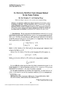
5 Results for a 2D Convective-Diffusive Problem A computational code has been developed for solving linear systems resulting of application of LSFEM to convection–diffusion problems. A test case presented by [5] was solved and the results are presented. The problem is a reverse flow in a cavity, illustrated in Figure 1. The domain is: −1 ≤ x ≤ 1; 0 ≤ y ≤ 1 . The velocity profile is known and defined as:

1. Assume an initial value for U αr ; 2. Calculate the residue Eαr as

Eαr = Fα − Kαβ U βr = Fα − Fα

(68) (69)

8. Calculate the correction factor, b r +1

(67)

(

(64a)

= u 2 y 1 − x2

with

);

(

v= −2 x 1 − y 2

)

(72)

E

Fαr = U f nδ nα e =1

and e f n = knm ume

(64c)

3. Define an auxiliary variable Pαr

:

Pα = Eα r

The inlet of the flow is in the region −1 < x < 0 , and exit is in the region 0 < x < 1 . With the velocity specified, the problem consists in solving a transport equation for the temperature field similar the system defined in Equation (22). The system of equations discretized in time has the form:

(64b)

r

(65)

n +1

T  ∂T ∂T   − +v  + α  u ∂y   ∂x  ∆t n +1 α  ∂q x ∂q y    − f n = 0 − + ∂y  Pe  ∂x

4. Calculate the residue in the iteration r: r = Eαr K= αβ Pβ

E

H nδ nα U e =1

(66a)

with e H n = knm Pmr

(66b)

5. Calculate the correction factor a r :

E-ISSN: 2224-3429

51

Volume 9, 2014

(73)



∂T n+1 =0 ∂x ∂T n+1 n +1 qy − =0 ∂y

q xn+1 −

matrix would be 39123 by 39123, if the complete system was assembled. In each element, there will be 27 degrees of freedom. Only the element matrix needs to be assembled, element by element, in the PCG-EBE procedure of solution. The results obtained from the computational code are presented in the Figure 2(a) for several numbers of Péclet. These results agree well qualitatively with results from [5]. In Figure 2(b), their results from Winterscheidt & Surana are compared with the results from [13]. It is observed that for high number of Pèclet, the convection is dominat as expected.

(74) (75) n

T  ∂T ∂T   − f =  + (1 − α ) u +v t x y ∆ ∂ ∂    n (1 − α )  ∂q x ∂q y    + q ''' − + ∂y  Pe  ∂x n

(76)

2,0

Pe = 10 Pe = 100 Pe = 500 Pe = 1e+3 Pe = 1e+4 Pe = 1e+5 Pe = 1e+6

θ

1,5

1,0

0,5

Figure 1- Geometry of the cavity and essential characteristics of the test-problem.

0,0

In the Equations (73) to (76), 0 ≤ α ≤ 1 is a parameter of time scheme discretization. The boundary conditions for solution of Eqs. (73) to (75) are:

T = 1 + tanh[10(2 x + 1)] ; −1 < x < 0;

−1, 0 ≤ y ≤ 1 x =  T = 1− tanh(10)  y = 1, − 1 ≤ x ≤ 1  x = 1, 0 ≤ y ≤ 1  ∂T = 0 ; 0 < x < 1; ∂y

y= 0

y =0

0,0

0,4

0,6

0,8

1,0

x

Figure 2 (a) – Temperature profiles at the cavity exit for several numbers of Pe.

(77a)

(77b, c, d)

(77e)

With the boundary conditions specified the values T will be nule in x = ±1 and y = 1 and approximately 2 in the origin of the coordinate system. The domain was discretized by a mesh of 80 by 40 elements in the X and Y axes, respectively, in a total of 3200 nine node quadrilateral elements. This corresponds to a total of 13041 of nodes in the mesh. Since there are 3 degrees of freedom by node, the total of unknowns will be approximately 39123, and the dimension of the global

E-ISSN: 2224-3429

0,2

Figure 2 (b) – Temperature Profiles at the cavity exit for several numbers of Pe .

52

Volume 9, 2014



temperature surfaces and isotherms are shown from Figures 4 to 12. Figures show temperature surfaces and isotherms, seen from X, Y and Z plans equal to 0.5. Therefore, isotherms in graphs are seen from the cuts at the respective X, or Y or Z plans.

6 Results for Tridimensional ConvectiveDiffusive Problems In this simulation, tests with a uniform mesh with 1000 elements (9261 points), corresponding to 10 divisions in each edge, were performed. Following [14], three different profiles of velocity were imposed: Case 1, Case 2 and Case 3, being based into. They are: 1

= ; V Case 1: U = 2

1

; V Case= 2: U = 3

1 = ; W 0; 2

(78)

1 −1 = ; W ; 3 3

(79)

T 0.95 0.9 0.85 0.8 0.75 0.7 0.65 0.6 0.55 0.5 0.45 0.4 0.35 0.3 0.25 0.2 0.15 0.1 0.05

1

0.8

0.6

1 = ; W 3

1 3

T

Case= 3: U

1 = ; V 3

;

(80)

0.4

0

0.2

0.5 1

Z

0

For the three cases, the boundary are illustrated in Figure 3. For each case, it has been kept the same boundary conditions and profile of velocity was varied according to [14], in order to analyse the influence of flow direction.

0.8 0.6

Y

0.4 0.2 0

1

Figure 4 – Distribution of temperature in X = 0.50 plan with Pe = 10, Case 1. T

1

0.8

0.6

T 0.4

0.2 0 0 1 0.5

0.8 0.6

Y

0.4 0.2 0

Figure 3 – Geometry and boundary conditions for tridimensional problems.

Z

0.95 0.9 0.85 0.8 0.75 0.7 0.65 0.6 0.55 0.5 0.45 0.4 0.35 0.3 0.25 0.2 0.15 0.1 0.05

1

Figure 5 – Distribution of temperature in X = 0.50 plan with 2

Pe = 10 , Case 1.

Convection-Diffusion in a Cubic Cavity (Case 1) The temperature profile in the Case 1, for parallel flow to X-Y plan in a cubic cavity, was obtained for Pe = 10, 102, 103, 104, 105, 106, 107, 108 and 109. Results of

E-ISSN: 2224-3429

53

Volume 9, 2014



T 0.95 0.9 0.85 0.8 0.75 0.7 0.65 0.6 0.55 0.5 0.45 0.4 0.35 0.3 0.25 0.2 0.15 0.1 0.05

T 1

0.8

0.6

0.2 0

0

0.8

0.6

T

T 0.4

1

1 0.9 0.8 0.7 0.6 0.5 0.4 0.3 0.2 0.1 0

0.4

0.2

0

0 1

1

0.5 0.8

0.8

Z

0.5

0.6

0.6

X

0.4

0.4

Y

Z

0.2

0.2 0

1

1

0

Figure 6 – Distribution of temperature in X = 0.50 plan with Figure 8 – Distribution of temperature in Y = 0.50 plan with Pe = 102, Case1.

4

Pe = 10 , Case 1

For low numbers of Pèclet, as can be observed at Figures 4 and 5, the temperature fields don´t present any apparent oscillations. For high numbers of Pèclet, some oscillations appear in the solutions a. As the method should stabilize the solution, probably the causes of oscillation maybe due to the gross mesh or for the fact of imposing the direction fo the flow not aligned with the mesh. But, they are speculations that must be more profoundly and well verified. Anyway, the solution has always converged.

T

1

0.8

0.6

T 0.4

0.2

T

1

0.8

0.6

T 0.4

0.2

0 0 1 0.8 0.6

0.5

X

0.4 0.2 0

Z

0

0 1

0.985914 0.95 0.9 0.8 0.7 0.6 0.5 0.4 0.3 0.2 0.15 0.1 0.05 0.020547 0.0094199 0.00377464 0.00101113 0.000229279

0.8 0.5

0.6

X

Z

0.4 0.2 0

1

Figure 9 – Distribution of temperature in Y = 0.50 plan with Pe = 104, Case1.

Now, some tridimensional graphs cuts in plans Z = 0,5 are presented for Case1. The same trend of previous graphs is also observed from sights of Z plan. T

1

Figure 7 – Distribution of temperature in Y = 0.50 plan with Pe =10, Case 1.

1

0.8

In sequence, some tridimensional graphs and cuts in plans Y = 0.5 are shown. At sights from Y plan, it is observed that for number of Péclet 100, some disturbance regions next to the corners start appearing, which are going to be accentuating as Péclet’s number increases, as it can be observed at figures next, for Case1. In general, the same trend of previous graphs is also observed from the sights of Y plan.

0.6

T

E-ISSN: 2224-3429

0.95 0.9 0.85 0.8 0.75 0.7 0.65 0.6 0.55 0.5 0.45 0.4 0.35 0.3 0.25 0.2 0.15 0.1 0.05

0.4

1

0.5 0 1 0.5

Y

54

0

X

0.2

0.95 0.85 0.75 0.65 0.55 0.5 0.45 0.4 0.35 0.3 0.25 0.2 0.15 0.1 0.05

0

Volume 9, 2014



Figure10 – Distribution of temperature in Z =0.50 with Pe = 10, Case 1.

Convection-Diffusion in a Cubic Cavity (Case 2)

The boundary conditions are those illustrated ones in Figure 3. Temperature profile in Case 2, for a cubic cavity with 1000 elements, was obtained for Pe = 10, 102, 103, 104, 105, 106, 107 and 108. Temperature surfaces and isotherms in X, Y and Z = 0.50 of the cavity are illustrated in Figures from 13 to 21. In this case, until a number of Péclet equal to 103, solutions seem to be smooth with no visible disturbances at the corners. For a number of Péclet equal 104 we can observe some oscillation.

T 0.95 0.85 0.75 0.65 0.6 0.55 0.5 0.45 0.35 0.25 0.15 0.05

1

0.8

0.6

T 0.4

1

0.5

X

0.2

0 1 0.5

Y

0

0

T 0.95 0.9 0.85 0.8 0.75 0.7 0.65 0.6 0.55 0.5 0.45 0.4 0.35 0.3 0.25 0.2 0.15 0.1 0.05

Figure 11 – Distribution of temperature in Z =0.50 plan com Pe = 102, Case 1. 1

0.8

T 0.6

0.6

T 0.4

1

0.5

0

0 0.2

0

0.5 1 0.8 0.6

Y

0.4 0.2

1

0

Figure 13. – Distribution of temperature in X = 0.50 plan with Pe = 10, Case 2.

X

0.2

0.4

Z

0.8

1 0.9 0.8 0.7 0.6 0.5 0.4 0.3 0.2 0.1 0

T

1

1 0.5

Y

0

0

Figure 12 – Distribution of temperature in Z =0.50 plan with Pe = 104, Case 1.

T

Analysis of Figures from 4 to 12 shows that, for low numbers of Péclet, qualitative the behavior is simulated; however, when the numbers of Péclet increases, oscillations start appearing at solution, which can occur because the mesh is not enough refined. The computers used for simulation were of low capacity of processing, and therefore, it was not possible to use very fine meshes. For these simulated cases, results took until 36 hours of running time to be obtained. It is probable that the problem is already characterized as a predominantly convective for Pe=104, which can also be the cause of oscillation. But, the same phenomenon can occur with upstream and exponential schemes.

0.8

0.6

T

E-ISSN: 2224-3429

1

0.4

0.2 0 0 0.5

1 0.8 0.6 0.4

Y

0.2 0

1

Z

0.95 0.9 0.85 0.8 0.75 0.7 0.65 0.6 0.55 0.5 0.45 0.4 0.35 0.3 0.25 0.2 0.15 0.1 0.05

Figure 14. – Distribution of temperature in X = 0.50 plan with Pe = 102, Case 2.

55

Volume 9, 2014



1

0.8

T 0.4

0

0.2

0.5

Z

0 1 0.8 0.6

Y

0.4 0.2 0

1

T

0.95 0.9 0.85 0.8 0.75 0.7 0.65 0.6 0.55 0.5 0.45 0.4 0.35 0.3 0.25 0.2 0.15 0.1 0.05

0.95 0.9 0.85 0.8 0.75 0.7 0.65 0.6 0.55 0.5 0.45 0.4 0.35 0.3 0.25 0.2 0.15 0.1 0.05

1

0.8

0.6

T

0.6

T

0.4

0.2

0

0 1 0.8 0.5

0.6

X

0.4

Z

0.2 1

0

Figure 15 – Distribution of temperature in X = 0.50 plan with Pe = 104, Case 2.

Figure 17 – Distribution of temperature in Y = 0.50 plan with Pe = 102, Case 2.

At Figures from 16 to 18, temperature surfaces and isotherms seen from Y = 0.5 plan are shown. None oscillations at solutions are observed. From the Figure 19, sights from Z =0.5 plan can be viewed.. In the Case 2, the obtained results seem to be better than those of Case 1, showing that direction of speed field has a great influence on the convection-diffusion process. Even for Peclet’s high numbers, oscillations are almost inexistent.

T 0.95 0.9 0.85 0.8 0.75 0.7 0.65 0.6 0.55 0.5 0.45 0.4 0.35 0.3 0.25 0.2 0.15 0.1 0.05

1

0.8

T

0.6

0.4

0.2

T

1

0.8

T

0.6

0.4

0.2

0 1

0 0.2 0.4

X 0.5

0.6 0.8 0

1

Z

0

0.95 0.9 0.85 0.8 0.75 0.7 0.65 0.6 0.55 0.5 0.45 0.4 0.35 0.3 0.25 0.2 0.15 0.1 0.05

1 0 0.2 0.4

X 0.5

Z

0.6 0.8 0

1

Figure 18 – Distribution of temperature in Y = 0.50 plan with Pe = 104, Case 2. T

1

0.8


0.6

T 0.4

0.2

0

0.5 1 0.8

0.6

0.4

Y

0.2

0

0

X

1

0.95 0.9 0.85 0.8 0.75 0.7 0.65 0.6 0.55 0.5 0.45 0.4 0.35 0.3 0.25 0.2 0.15 0.1 0.05

Figure 19 – Distribution of temperature in Z = 0.50 plan with Pe = 10, Case 2.

E-ISSN: 2224-3429

56

Volume 9, 2014



T

0.8

0.6

T 0.4 1

0 1 0.5

Y

0

0

1

0.8

0.6

0 0.4

0.2

Z

0.5

X

0.2

T

T

1

0.95 0.9 0.85 0.8 0.75 0.7 0.65 0.6 0.55 0.5 0.45 0.4 0.35 0.3 0.25 0.2 0.15 0.1 0.05

0.5

0

0.95 0.85 0.75 0.65 0.55 0.45 0.35 0.3 0.25 0.2 0.15 0.1 0.05

0 1


0.5

Y

1


T

T

0.5

0.5

0 1 0.8 0.6

Y

0.4 0.2 0

0

X

1

T

1

0.8

0.6

T

1

0.95 0.9 0.85 0.8 0.75 0.7 0.65 0.6 0.55 0.5 0.45 0.4 0.35 0.3 0.25 0.2 0.15 0.1 0.05

0 0.4

0.2

Z


0.95 0.85 0.75 0.65 0.55 0.45 0.4 0.35 0.3 0.25 0.2 0.15 0.1 0.05

0.5 0 0 0.5 1

Y

1


Convection-Diffusion in a Cubic Cavity (Case 3) For the Case the results are showed in next figures. The boundary conditions are illustrated at Figure 3. Temperature fields are shown in Figures from 22 to 27. In this case, we don´t have simulations for high number of Pèclet. The simulations are for Pèclet equal to 20 and 100. For these low numbers of Pèclet the solutions seems to be free os oscillations.

T 1

0.8

0.6

T 0.4

0.2

0 0

0.95 0.85 0.75 0.65 0.55 0.45 0.35 0.25 0.2 0.15 0.1 0.05

1 0.8

0.5

0.6

X

Z

0.4 0.2 0

1


E-ISSN: 2224-3429

57

Volume 9, 2014



7 Conclusions LSFEM has been applied for solution of first order partial differential equation systems in the case bi and tridimensional heating transfer problems. It is always possible, by using auxiliary variables, such as heat flows or vorticity, or tension, to write partial differential equations of second order as a partial differential equations system of first order. LSFEM application always results into a symmetrical and defined positive algebraic system, independently of the form original differential operator. This kind of system is appropriately solved by conjugate gradient methods. Resultant algebraic systems have been solved by the preconditioned conjugate gradient method, with a preconditioner element by element, eliminating the need for a global matrix assembly. Globaly only vectors are used for storage of variables. All operation with matrices are performaed at element level. In these simulations, Quadratic Quadrilateral Finite Elements of nine nodes were used, for bidimensional problems and quadratic hexahedrons with twenty-seven nodes in the tridimensional cases. Results from simulations have presented the expected behavior; however, in the tridimensional cases, when Peclet’s number increases, there are still certain oscillations in the solutions, mos t probably due to the utilization of coarse meshes, once that well refined meshes were not able to be achieved, because of the utilized computational capacity. All of the simulations were performed through microcomputers of medium capacity of processing.

T 1

0.8

0.6

T 0.4

0.2

0 0 1 0.8

0.5

0.6

X

0.95 0.85 0.75 0.65 0.55 0.5 0.45 0.4 0.35 0.25 0.15 0.05

Z

0.4 0.2 0

1


T

1

0.8

0.6

T

1

0.4

0.5

X

0.2

0 1

0.95 0.85 0.75 0.65 0.55 0.45 0.35 0.3 0.25 0.2 0.15 0.1 0.05

0.5

Y

0

0


References [1] O. C. Zienkiewicz, R. L. Taylor and E. P. Nithiarasu, The finite element method for fluid dynamics. Editora Elsevier, 2005.

T

1

0.8

T

0.6

1 0.4

0.2

X

0.5

0.95 0.85 0.75 0.65 0.55 0.5 0.45 0.4 0.35 0.25 0.15 0.05

[2] J. N. Reddy, An introduction to the finite element method. Second Edition, McGraw-Hill, Inc., New York, 1993. [3] G. Dhatt and G. Touzot, The Finite Element Method Displayed. John Wiley and Sons, Chichester, 1978. [4] B. N. Jiang, The Least-Squares Finite Element Method: Theory and Aplications in Computational Fluid Dynamics and Electromagnetics, Springer, New York, 1998.

0 0 0.5 0

1

Y


E-ISSN: 2224-3429

58

Volume 9, 2014



equations. Journal of Computational Physics, 190, 523549, 2003.

[5] K. S. Surana and D. Winterscheidt, p-version leastsquares finite element formulation for convection diffusion problems. International Journal for Numerical Methods in Engineering, Vol 36, p.111-133, 1993.

[11] P. Bolton and R. W. Thatcher, A least-squares finite element method for the Navier-Stokes equations. Journal of Computational Physics, 213, 174-183, 2005.

[6] K. S. Surana and D. Winterscheidt, p-version leastsquares finite element formulation for two-dimensional, incompressible fluid flow. International Journal for Numerical Methods in Fluids, Vol 18, p.43-69, 1994.

[12] A. Bejan, Transferência de Calor, Editora Edgard Blücher Ltd., Brazil, 1996. (in portuguese) [13] T. J. Chung, Computational Fluid Dynamics. Cambridge University Press, 2002.

[7] P. B. Bochev and M. D. Gunzburger, Analysis of least squares finite element methods for the stokes equations. Mathematics of Computation, vol. 63, 208, 479-506, 1994.

[14] R. M. Smith and A. G. Hutton, The Numerical Treatment of Advection: a Performance Comparison of Current Methods Numerical Heat Transfer, Part B. An International Journal of Computation and Methodology, 1521-0626, Volume 5, Issue 4, pg. 439 – 461, 1982.

[8] C. B. Bell and K. S. Surana, A space – time coupled pversion least-squares finite element formulation for unsteady two-dimensional navier – stokes equation. International Journal for Numerical Methods in Engineering, Vol 39, p. 2593-2618, 1996.

[15] B. Ledain Muir and B. R. Baliga, Solution of ThreeDimensional Convection-Diffusion Problems Using Tetrahedral Elements and Flow-Oriented Upwind Interpolation Functions. Numerical Heat Transfer, V. 9, p 143-162, 1986.

[9] A. Duster, H. Broker and E. Rank, The p-version of the finite element method for three-dimensional curved thin walled structures. International Journal for Numerical Methods in Engineering, 52, 673-703, 2001. [10] J. P. Pontaza and J. N. Reddy, Spectral hp leastsquares finite element formulation for the Navier_Stokes

E-ISSN: 2224-3429

59

Volume 9, 2014

Stabilized Least Squares Finite Element Method for 2D and ... - WSEAS

Stabilized Least Squares Finite Element Method for 2D and ... - WSEAS

Suggest Documents

Least Squares Finite Element Method for 3D Unsteady ... - WSEAS

least-squares finite element methods for

LEAST-SQUARES FINITE ELEMENT METHODS FOR QUANTUM

least-squares finite element method - Purdue Math - Purdue University

Adaptive mixed least squares Galerkin/Petrov finite element method ...

Discrete least-squares finite element methods - arXiv

least-squares finite element methods for - Mathematical and Statistical

least-squares finite element methods for - Mathematical and Statistical

least-squares finite element methods for - Mathematical and Statistical ...

least-squares finite element methods for - Mathematical and Statistical ...

least-squares finite element methods for - Mathematical and Statistical ...

on least-squares finite element methods for the poisson ... - CiteSeerX

An Absolutely Stabilized Finite Element Method - American

least-squares finite element methods for - Semantic Scholar

LEAST-SQUARES FINITE ELEMENT METHODS FOR - University of ...

least-squares finite element methods for - Semantic Scholar

Stabilized finite element method for heat transfer and ...

NURBS based least-squares finite element methods ...

a second order control-volume finite-element least-squares strategy ...

Least-squares finite element methods - People - Florida State ...

finite element methods of least-squares type - CiteSeerX

A stabilized finite element method for calculating ... - Geosci. Model Dev.

A Stabilized Mixed Finite Element Method for Thin Plate Splines

A Stabilized Cut Streamline Diffusion Finite Element Method for ...