2). Calculate a new control input that minimizes the cost function. 3) ...... M.E.
Degree in ... He is working as faulty in T.R.R.College of Engg.J.N.T.U.Hyd.
©2007 Institute for Scientific Computing and Information
INTERNATIONAL JOURNAL OF INFORMATION AND SYSTEMS SCIENCES Volume 3, Number 1, Pages 1-15
NEURAL GENERALIZED PREDICTIVE CONTROLFOR REAL TIME APPLICATIONS
D. N. RAO, M. R. K. MURTHY, S. R. M. RAO AND D. N. HARSHAL
Abstract A novel method of recursive formulation is embedded in Neural Generalized Predictive control (NGPC) algorithm and subsequent on-line control based on extended memory
techniques (EMT) are investigated. The utility of both recursive and EMT are
integrated and demonstrated for a typical nonlinear model plant. The simulation results show that it is a viable approach with good performance for real time control. Key Words, Recursive formulation, Neural Generalized predictive control, extended memory adaptation, real time control.
1. Introduction Generalized predictive control (GPC) belongs to the class of digital control methods called Model-Based Predictive Control (MBPC) and was introduced by Clarke and his Co-workers in 1987[1, 2]. GPC is known to control non-minimum phase plants, open loop unstable plant and plants with variable or unknown dead time and originally developed with linear plant predictor model. For a large number of Systems a linearising approach is acceptable, any relatively small non linearities being effectively linearised by the controller [2, 6]. In order to obtain an improved control over systems with small non linearities or to deal with Systems with Stronger nonlinearties, whilst obtaining the benefits of a neural network, it is necessary to take account of the non linearities in an appropriate way [2]. The ability of GPC to make accurate predictions can be enhanced in a neural network is used to learn the dynamics of the plant [3] [4]. This application combines the advantages of predictive control and neural net work, Known as Neural generalized predictive control (NGPC), developed by Donald Soloway, 1996[5]. Embedding a nominal linear model into the neural network is a suitable way to solve the problem of an open-loop unstable plant. For highly nonlinear plants or plants operating over a large set of condition, a method of breaking an input space into multiple linear regions is sometimes employed. This technique using NGPC is studied in [6]. Neural networks offer a flexible structure that can map arbitrary nonlinear functions, making them ideally suited for the modeling and control of complex nonlinear systems [7], [8]. They are particularly appropriate for multivariable applications, where they can readily characterize the interactions between different inputs and outputs. The training of these networks in NGPC can be performed off-line and subsequently be augmented as Received by the editors March 15, 2006 1
2
D. RAO, .M. MURTHY, .S. RAO AND D. HARSHAL
part of an on-line adaptive scheme. A further benefit is that the neural architecture is inherently parallel, distributed and has the potential for real time implementation. The goal of this paper is to show that, provided with appropriate accelerated adaptation techniques and control structures [9], neural networks can be used to adaptively control a wide range of nonlinear processes at a useful level of performance. The method proposed consists of a novel identification technique based on extended memory adaptation (EMT) and an efficient implementation of the predictive control based on a nonlinear programming algorithm. The organization of the paper is as follows: This paper has discussed issues concerning the NGPC with recursive formulation with extended memory adaptation integrated technique. In section 2 the recursive formulation for NGPC (RNGPC) investigated. In section 3 the proposed extended memory technique (EMT) investigated. In Section 4 the RNGPC integrated with EMT algorithm explained. Section 5 shows the simulation results of combined techniques demonstrated. Conclusions are presented in section 6. 2. Recursive formulation for NGPC The block diagram of the NGPC is shown in figure 1. Its consists of four components: The plant to be controlled , a neural network model for prediction, a tracking signal that specifies the desired position ,and the cost function minimization(CFM) algorithm that calculates the current command to produce the desired position. To derive the control law considers the performance index J over the entire prediction horizon 'N' as: NU ⎫ ⎧ N2 2 J(N1, N 2 ) = E ⎨ ∑ (y(n + j) − w(n + j)) + ∑ λ( j)[ ∆u(u + j − 1)]2 ⎬ j=1 ⎭ ⎩ j= N1
(1)
Where N1 is the minimum costing horizon, N2 is the maximum costing horizon, NU is the control horizon, Ym is the desired tracking trajectory, Wn is the predicted output of the model, λu is the control input weighting factor is performance error function. By minimizing the above performance Index one can get the incremental control vectors: −1 U% = ( GT G + λ I ) GT (W − f )
(2)
and control input given as: u ( n ) = u ( n − 1) + ∆u ( n ) . The equations (1) and (2) are fundamental equations of NGPC scheme. To derive the control law considers the performance index J over the entire prediction horizon 'N' as: N2
Nu
J ( N1 , N 2 ) = E{ ∑ ( y ( n + j ) − w ( n + j ) ) + ∑ λ ( j )[∆u ( u + j − 1)]2 } j = N1
2
j =1
(3)
NEURAL GENERALIZED PREDICTIVE CONTROL
3
Figure 1: Block diagram of NGPC scheme
The NGPC algorithm operates in two modes, prediction and control. The main steps of the NGPC algorithm are: 1)
Starting with the previously calculated control input, u (n) predicts the performance of the plant for the specified horizon using the model. The value of the horizon is determined through a priori tuning.
2)
Calculate a new control input that minimizes the cost function.
3)
Repeat steps1 and 2 until desired minimization is achieved, and send "the best" control input as the new u (n).
4)
Repeat for each time step.
The original NGPC requires the inversion matrix whose size depends upon the horizon. This can be seen as the main drawback of this method. And it was mentioned that control horizon (NU) determines the size of the matrix to be inverted, yet it is time consuming when the output horizon (N2) is increased, even to calculate iteratively. They did not propose any method to avoid inversion as such and they did not also suggest any modification in the original NGPC method. Here is a simple recursive scheme is proposed, which calculates the incremental control value recursively in NGPC. The neural network’s natural recursion adding with proposed recursive control increments results the more viable algorithm to predict the Plant’s dynamics especially smaller non linear plants.
4
D. RAO, .M. MURTHY, .S. RAO AND D. HARSHAL
Currently, there is no systematic way to determine the values for the four tuning parameters N1, N2, Nu and λ u for a non-linear system. The recursive formulation is very simple and straightforward to implement and also does not require the priori specification of the prediction horizon. This property is very useful in practical implementation of NGPC as at each sampling instant prediction horizon is automatically adjusted to a suitable value depending on the termination criterion used. The recursive NGPC also avoids the inverse of the control matrix. Whenever the horizon is increased, one need not have to repeat the whole procedure. On the contrary one has to calculate only the extra terms to be added to the previous control value when the control horizon is increased by utilizing the previous values without much computational effort. It is always advantageous to have a recursive scheme from the point of view of implementation. In this section a simple recursive solution is given which is generalized for varying NU and N.
Consider for NU=1 and a particular horizon N = (N2) As seen from NGPC gives that:
(
~ G = [g 0 , g1, g 2 ....g n ]T and U = G T G + λI
)
−1
G T (W − f )
For convenience let W − f = a
(
~ U = G T G + λI
)
−1
G Ta ,
where
G T = [g 0 , g1, .....g n −1 ]
[
n −1
G Ta ∑ g i a i +1
Therefore
Similarly
Dividing by
n−1 i=0
Therefore
Similarly
]
GTG = g20 + g12 + g22 + ......... g2n−1 =∑g2i
i =0
n −1 ⎛ n −1 ⎞ ~ U n = ∑ g i . a i +1 / ⎜ ∑ g 2i + λI ⎟ i =0 ⎝ i =0 ⎠ , this gives
n −1 ⎡ n −1 2 ⎤ ~ + λ g I U = g i a i =1 ∑ ∑ i n ⎢ ⎥ i =0 ⎣ i =0 ⎦
n ⎛⎛ n 2 ⎞⎞~ ⎜⎜ ⎜ ∑ g i + λI ⎟ ⎟⎟U = g i . a i +1 ∑ n +1 i =0 ⎠⎠ ⎝ ⎝ i =0
⎞ ⎛ ⎛ n −1 2 ⎞ ⎜⎜ ⎜ ∑ g i ⎟ + λ I ⎟⎟ ~ ⎠ ⎠ and writing in terms of U n gives as: ⎝ ⎝ i=0 ⎛ ⎛ n −1 2 ⎞ ⎞ ~ ⎛ ⎛ n +1 2 ⎞ ⎞ ~ ⎜⎜ ⎜ ∑ g i ⎟ + λI ⎟⎟ U ⎜ ⎟ n +1 = ⎜ ⎜ ∑ g i ⎟ + λI ⎟ U n + g n . a n +1 ⎝ ⎝ i =0 ⎠ ⎠ ⎝ ⎝ i =0 ⎠ ⎠
(3)
5
NEURAL GENERALIZED PREDICTIVE CONTROL
Let
g n . a n +1 = K11
and ⎛⎛ n 2 ⎞ ⎞ ~ ⎛ ⎛ n −1 2 ⎞ ⎞ ~ ⎜⎜ ⎜ ∑ g i ⎟ + λI ⎟⎟ U ⎜ ⎟ n +1 = ⎜ ⎜ ∑ g i ⎟ + λI ⎟ U n + K11 0 i i 0 = = ⎝ ⎠ ⎝ ⎠ ⎝ ⎠ ⎝ ⎠
therefore
For NU = 2
With the same notation: ⎡⎛ n−1 2 ⎞ ⎢⎜∑gi ⎟ + λI ⎢⎝ i=0 ⎠ GTG+ λI = ⎢ ⎢ ⎢n−2 ⎢∑gi gi+1 ⎣i=0
(
⎞ ⎛ n −3+ j ~ D n U n 2( j) = ⎜⎜ ∑ g 2i + λI ⎟⎟ i = 0 ⎠ ⎝
And
(4)
)
⎞ ⎛ n− j ⎜⎜ ∑ g i a i + j ⎟⎟ i = 0 ⎠ ⎝
⎤ ⎡ n −1 ⎤ ⎥ ⎢∑ gi a i +1 ⎥ i=0 ⎥ i =0 ⎥ ⎥ G T a = ⎢⎢ ⎥ ⎥ ⎢ n −2 ⎥ ⎛⎛n−2 2 ⎞ ⎞ ⎥ ⎢∑ g a ⎥ ⎜⎜⎜∑gi ⎟ + λI⎟⎟ ⎥ i i +2 ⎢⎣ i =0 ⎥⎦ ⎝⎝ i=0 ⎠ ⎠ ⎦ n−2
∑g g i
i+1
(
)
⎛ n −3 + j − ⎜⎜ ∑ g i a i +3− j ⎝ i =0
n −2
∑g i =0
i
⎞ g i +1 ⎟⎟ ⎠
(5)
Where ⎞ ⎛ ⎛ n −1 ⎞ D n = ⎜⎜ ⎜ ∑ g 2i ⎟ + λI ⎟⎟ ⎠ ⎝ ⎝ i =0 ⎠
⎞ ⎛ n −2 ⎛ ⎛ n −2 2 ⎞ ⎞ ⎜⎜ ⎜ ∑ g i ⎟ + λI ⎟⎟ − ⎜ ∑ g i g i +1 ⎟ ⎠ ⎠ ⎝ i =0 ⎝ ⎝ i =0 ⎠
2
⎛ n − 2+ j − ⎜⎜ ∑ g i a i +3 j . ⎝ i =0
n −1
∑g i =0
i
⎞ g i +1 ⎟⎟ ⎠
(6)
This can be written as ⎛ ⎛ n −3 + j 2 ⎞ ⎞ ⎜ ⎜⎜ ∑ g i ⎟⎟ + λI + g 2n −2+ j ⎟ ⎜ i =0 ⎟ ⎠ ⎝⎝ ⎠
⎛ n− j ⎞ ⎜⎜ ∑ g i a i + j + g n + i − j a n +1 ⎟⎟ ⎝ i =0 ⎠
⎛ n −3 + j ⎞ ⎛ n −2 ⎞ − ⎜⎜ ∑ g i a i +3 j + g n −2+ j . a n +1 ⎟⎟ ⎜ ∑ g i g i +1 g n −1 g n ⎟ ⎠ ⎝ i =0 ⎠ ⎝ i =0
(7)
Dividing by and manipulating ⎡D ⎤ ~ ~ U n +11( j) ⎢ n +1 ⎥ = U n 2( j) + K j, nu ⎣ Dn ⎦
(8)
⎛ ⎛ n −3+ j ⎞ ⎞ ⎞ ⎛n−2 ⎛n−3+j ⎞ k j, nu = ⎜⎜ ⎜⎜ ∑ g 2i ⎟⎟ + λI ⎟⎟ (g n +1j a n +1 ) − ⎜⎜ ∑gi ai+3j gn gn−1⎟⎟ +⎜ gi gi+1 an+1 + gn−2+j an+1 gn gn−1⎟ ⎠ ⎝ i=0 ⎝ i=0 ⎝ ⎝ i =0 ⎠ ⎠ ⎠
∑
6
D. RAO, .M. MURTHY, .S. RAO AND D. HARSHAL
(9) Where
D n +1 can be written in terms of D n as: ⎛ n − 2+ j ⎞ D n +1 = D a + ⎜⎜ ∑ g2i + λI ⎟⎟g 2n −1+ j + g 2n −1+ j ⎝ i =0 ⎠ ⎛ ⎛ n −3+ j ⎞ 2⎞ − ⎜⎜ 2⎜⎜ ∑ g i g i +1 ⎟⎟ (g n −2+ j g n −1+ j ) + (g n −2+ j g n −1+ j ) ⎟⎟ ⎠ ⎠ ⎝ ⎝ i =0
(10)
2.1The same can be extended using the partitioned matrix method as given below: Let the matrix be defined as: n−2 n −nu ⎡ n−1 2 ⎤ g i g i+1 .... ∑ g i g i+nu −1 ⎥ ∑ ⎢((∑ g i ) + λI ) i =0 i =0 ⎢ i=n0−2 ⎥ n−2 n −nu 2 ⎢ g i g i +1 ((∑ g i ) + λI ) .... ∑ g i g i+nu −2 ⎥ ⎢ ∑ ⎥ i =0 i =0 i =0 ⎢ ⎥ .. .. .. n − nu n −nu ⎢ n−nu ⎥ 2 ⎢ ∑ g i g i+nu −1 g i g i +nu −2 .... (( ∑ g i ) + λI )⎥ ∑ ⎢⎣ i =0 ⎥⎦ i =0 i =0
(11)
This can be written in a partitioned matrix form as ⎡L Q ⎤ Bi = ⎢ i i ⎥ ⎣ Ri Si ⎦
With L11 = ((
n −1
∑g i =0
2 i
(12)
) + λI ) , and dim Bi = (i, i) i ∈ (2, NU), dim Li = (i-1, i-1),dim Qi
= (i-1, 1), dim Ri = (1, i-1)
and
dim Is = (1, 1), for i = 2, 3, .NU.
From the quantities Q, R, S as:
[
]
n −1
Ri = Ri j −1 , Ri j − 2 ....Ri2 , Ri1 and Ri j = ∑ g i g i + j i =0
n − nu
Qi = RiT and S i = (( ∑ g i ) + λI ) i =0
2
7
NEURAL GENERALIZED PREDICTIVE CONTROL
and the inversion can be calculated by the following formula.
( (
)
(
) )
−1 ⎡ L − Q S −1 R −1 − Li − Qi Si−1 Ri Qi Si−1 ⎤ i i i i ⎥ B =⎢ −1 −1 ⎢⎣ − Si Ri Pi −1Qi Ri Pi −1 ⎥⎦ Si Ri Pi −1Qi −1 i
)
(
(13)
The general equation for N and NU for changes both in N and NU can be written as shown below.
DijYˆij = Di −1 j
j
∑g r =1
~
i − r −1
j
U (r ) + f i −1 + ∑ g i −r K rj + Di f i
(14)
r =1
where i ∈ 3 to N+1 the output horizon, i ∈ 2 to NU the control horizon. The above equation can be verified as shown as (10)
⎛ ⎛ n−3+j ⎞ ⎛ n − 2+ j ⎞ 2⎞ D n +1 = D a + ⎜⎜ ∑ g2i + λI ⎟⎟g 2n −1+ j + g 2n −1+ j − ⎜⎜2⎜⎜ ∑gi gi+1 ⎟⎟ (gn−2+j gn−1+j ) + (gn−2+j gn−1+j ) ⎟⎟ ⎠ ⎝ i =0 ⎠ ⎠ ⎝ ⎝ i=0 From the above equation 8 it is observed that whenever the output horizon is increased ~ from N to N+1, ~ U n+1 can be calculated in a recursive way from U n and when the control horizon is increased from 2,3..... NU, the same can be extended. The outputs y (n), y (n+1).....etc. using the Neural Network model can be obtained. Example: Consider second order non-minimum phase system:
y (t) - 1.6y (t-1) + 0.8y (t-2) = 0.5 u (t-1) + 1.5 u (t-2) Consider N2 = 5, NU = 2, W = 5. Using recursive algorithm:
⎡0.5 2.8 6.08 9.488 12.316 ⎤ GT = ⎢ ⎥ ⎣0.0 0.5 2.8 6.08 9.488 ⎦
⎞ ⎛ n − 3+ j ⎞ ⎛ n− j ⎛ n − 3+ j 2 ⎟ ⎜ ⎜⎜ ∑ g i ai +3− j ⎟ g λ I g a − + ∑ i ⎟ ⎜ ∑ i i+ j ⎟ ⎠ ⎝ i =0 ⎠ ⎝ i =0 ⎝ i =0
~ U n 2( j ) = D ⎜⎜
~ For λ = 1;W = 5; N = 5 , U n 2(1) = − 0.7279 ,
n−2
∑g i =0
i
⎞ g i +1 ⎟⎟ ⎠
~ U n 2(2) = 0.3259
When the horizon increases from N to N+1 calculate Kj, nu and add to the Un so that we can get Un+1 using equation (9) and substituting in equation (8) lead as: ~ ~ D n +1 U n +1 2( j) = D n U n ( j) + D n Kj, nu ,
8
we get
D. RAO, .M. MURTHY, .S. RAO AND D. HARSHAL
~ ~ U n +1 2(1) = −0.81, U n +1 2 (2) = 0.490
These results show that the process of inverse can be eliminated when ever the horizon increases. 3. Extended Memory Technique in NGPC A general model structure suitable for representing the dynamics of a wide range of nonlinear systems model defined by: y(k) = f(y(k-1),...,y(k-ny),u(k-d-1),...,u(k-d-nu))+e(k) (15)
where y (k) and u (k) are the sampled process output d represents the process dead-time and f (.) is an unknown nonlinear function to be identified. It is important to note a distinction between two different modes of operation of a trained neural network model. In eqn. (15), the network requires both input and output data from the process as inputs, and it predicts the process output a single time step into the future, yn (k). In this predictor structure, a trained network cannot, therefore, be used independently from the plant, or to provide long range predictions. These two tasks can be achieved by operating a trained network in the model structure: yn(k)= f(yn(k-l),...,yn(k-ny),u(k-d-1),...,u(k-d-nu))
(16)
where yn (k) is the model predicted output of the network. In eq. (16), the network is supplied with input data, u (k), and the network outputs, yn (k), are delayed and fed back to the network inputs to project predictions of the process output further into the future. The. difference between these two modes of network operation is illustrated in Figure 2 In off-line training it is difficult to assure the conditions for a good generalization of the neural networks hence the on-line training is always necessary in control applications. In fact, the training should ideally occur exclusively on-line, with the neural networks learning at high speed from any initial set of weights. In order to make neural control a viable alternative to industrial control of processes, there is a pressing necessity for efficient on-line training algorithms. The purpose of this section is to present a new technique, denoted Extended-Memory Technique (EMT), for improving the convergence characteristics of adaptive identification. To convert the learning procedure to an adaptive algorithm the single pattern generated by the tapped delay lines from the process sample at each time-step is applied to the NN to obtain a small increment of adaptation at each time-step as shown in Figure 3.
NEURAL GENERALIZED PREDICTIVE CONTROL
9
Figure 2. Switch in position A gives predictor & position B gives model operation.
To make the procedure adaptive over time the context of application of learning rule has been changed from batch to single pattern presentation environment. A Multiple-Input Multiple-Output model suitable for identification can be expressed in terms of θ (k), the set of unknown parameters, past values of the inputs and outputs, and modeling errors e (k):
y(k ) = f (θ (k ), y (k − 1),...,y (k − n y ), u (k − 1),..., u (k − nu )) + e(k )
(17)
Figure 3. Integration of extended-memory into the identification structure.
At time step k each weight wji, connecting the input of node i on each layer, to the output of node j on the preceding layer, is updated using:
10
D. RAO, .M. MURTHY, .S. RAO AND D. HARSHAL
w ji (0 ) = γ ji
(18)
+
where α ∈ R is the learning rate, 0 < β < 1 is the momentum factor, ei(k) is the back propagated error value corresponding to the input to the sigmoid function calculated for node i during the presentation of the pattern θ (k) derived from process time k. The addition of a momentum term in the learning rule can greatly accelerate convergence. The random variable γ ji is independently selected for each weight from a distribution with zero mean and small variance. This recursive equation is applied to each weight at each time-step k of the plant operation. A distinction should be made between iteration q and time step k. The updated weight wji (q, k) is calculated using the extended recursive equation set below:
w ji (0,0 ) = γ ji , w ji (0,0 ) = w ji (1, k − 1) w ji (q, k ) = w ji (q − 1, k ) + αe i (k ) + β(w ji (q − 1, k ) − w ji (q − 2, k ))
(19)
The method proposed retains some process patterns that can represent an approximation to the nonlinear process dynamics. The extended memory (EM) accepts a new pattern θ (k) from the process at each time step k and discards the oldest pattern θ (k-np). The EM elements θ (k), θ (k-l)... θ (k-np+l) are each used in nc cycles to update the weights at each time-step. The recursive equation set can be written as follows:
w ji (0,0 ) = γ ji ,
w ji (0,0 ) = w ji (1, k − 1)
w ji (q, k ) = w ji (q − 1, k ) + αe i (k ) + β(w ji (q − 1, k ) − w ji (q − 2, k ))
(20)
where: 1 is a cycle counter for nc cycles of the pattern memory which are performed at time step k , p indicated the time step origin of the pattern selected from the EMA is chosen in random order from its index range (k - np +1 , k). At each selection of p and execution of the recursion, the iteration count q is incremented, up to ncnp. By applying the supervised learning rule using all the patterns of the EM for learning at each time step, the rule drives the weight vector of the network towards one that minimizes the error corresponding to the approximate mapping represented in the EM patterns. The random order of presentation ensures that the sampled pattern order does not adversely affect the learning rule dynamics. The EM technique algorithm is summarized as follows:
NEURAL GENERALIZED PREDICTIVE CONTROL
1. 2. 3. 4. 5. 6. 7. 8.
11
Sample inputs and outputs of the process. Shift and update the TDL elements. If TDL are not full, restart at step 1 at next time step. Construct a training pattern from elements of TDLs and the latest process output sample. Execute neural network to calculate one-step ahead prediction. Insert the new pattern into the EM. If the EM size > np , remove the oldest pattern. Train network for nc cycles of up to np EM patterns presentation (randomized order).
4. Recursive NGPC with EMT techniques A schematic of neural generalized predictive control structure with EMT shown in fig. 4. Adaptive Neural Predictive Control with combined algorithm is as follows: 1. Sample inputs and outputs of the process. 2. Shift and update the TDL elements. 3. if TDL are not full, restart at step 1 at next time step. 4. Use the NN model to predict the estimate yn. 5. Construct a training pattern from elements of TDLs and the latest output sample. 6. Insert the new pattern in EM (if the EM size > np remove the oldest pattern). 7. Train network for nc cycles of up to np EM patterns (randomized order). 8. Use TDL values and proposed control actions to predict future process trajectory. 9. Evaluate performance objective function. 10. Improve proposed control actions and go to step 10, until optimized. 11. Output the control actions calculated for time-step k to the process.
Figure 4. Neural network (adaptive) predictive control scheme.
The adaptation of control strategy to the parameters changes of the model it is also considered. In this case the nonlinear model is constructed and a control strategy is
12
D. RAO, .M. MURTHY, .S. RAO AND D. HARSHAL
adapted minimizing a quadratic cost function in predictive control sense.
5. Simulation Results Simulation was carried out on a typical plant to demonstrate the utility of recursive formulation. A suitable criterion is used to terminate the recursion. One such criterion is standard deviation. Always this value is to be specified a priori based on the nature of the plant and accuracy required. So that the termination gets effected automatically, there by reducing the computational burden quite considerably. Apart from that, it provides with a means by which prediction horizon can be changed on-line, and this is admittedly, a very good feature which can be employed very advantageously. Cleary, the termination criterion enhances the utility of the recursive scheme. The horizon need not be specified a priori and wait till the same is over irrespective of the conditions obtaining in the system. This is very useful in practice since at each sampling instant a suitable value of the prediction horizon is automatically fixed to give a better convergence. In fact, this automatic assignment of the prediction horizon removes the uncertainty over the output convergence and hence in all the cases it has been found to improve the response. Consider the simulation plant (typical non linear plant) equation:
y(k)=0.6206y(k-1)+0.3785y(k-2)+0.0033u(k-1)–0.0088u(k-1)y(k-2) (21) The results obtained were in accord with those expected from using a predictive control methodology. It is seen that with no weighting of the control input good set-point tracking is achieved; however, the control input exhibits large fluctuations. For larger values of, movement of the manipulated variable is dampened at the expense of poorer set-point tracking. It was observed that increasing the prediction horizon had a number of desirable effects. Good set-point tracking was maintained, whilst the control effort was considerably reduced. These results demonstrate that improvements can be achieved with neural network in practice. This method is better than the other approaches due to fast adaptation and ability to address process nonlinearity. For time-varying processes, adaptation is the only means by which the performance of the controller can be maintained.
Table 1 Comparison between RNGPC and NGPC with EMT
RNGPC
NGPC
NU
Un
Yn
Un+1
Yn+1
2
-0.7279
4.224
-0.81
4.192
2
0.3259
5.11
0.49
4.9
3
-0.5646
4.3097
-0.6012
4.2914
3
-0.1866
5.2948
-0.0425
5.23
3
-0.0071
5.016
0.22315
5.32
2
-0.7304
4.226
-0.815
4.185
13
NEURAL GENERALIZED PREDICTIVE CONTROL
2
0.3281
5.081
0.5106
4.92
3
-0.5654
4.3092
-0.6128
4.285
3
-0.1872
5.2942
-0.0425
5.24
3
0.00716
5.014
0.2330
5.29
Table 2 Comparison between RNGPC and NGPC from point of view of CPU time with
EMT. No. of
Percentage
CPU Time
predictions
reduction
taken
2
60
40
129m.sec
3
59
40
127m.sec
2
150
-
141m.sec
3
150
-
147m.sec
Nu RNGPC
NGPC
Figure 5: Control performance using NGPC + EMT (Solid) and RNGPC +
EPA(dashed)with N1 = 1, N2 = 30, Nu = 2,
λ u = 0.05
(a) Large scale (b) Small scale
14
D. RAO, .M. MURTHY, .S. RAO AND D. HARSHAL
Figure 6: Control performance using NGPC (Solid) and RNGPC (dashed) with N1 = 1, N2 = 30, Nu = 2,
λ u = 0.005
(a) Large scale (b) Small scale
6. Conclusions A recursive solution is presented for the calculation of the control vector and the predicted output used in NGPC integrated with EMT schemes. This is very simple and straight forward to implement. This is very helpful in NGPC implementation, since the value of prediction horizon need not be specified in advance. It is automatically adjusted to a suitable value depending on the termination criterion. The recursive solution also does not require the Inversion of the control matrix at each sampling instant as is done in the original NGPC algorithm. Finally the utility of recursive solution is demonstrated with the help of simulation studies. A novel method is proposed to greatly accelerate the real time learning of input-output mappings by feed-forward neural networks. The method is superior due to recursively estimation and ability to address given plant. It is a viable control approach which can achieve good performance when applied to non linear plant.
REFERENCES
[1]D.W Clarke, C. Mohtadi and P.C. Tuffs, "generalized predictive control - Part I and Part II. The basic algorithm", Automation, Volume 23, 1987, PP 137 - 148 and PP 146 - 163. [2]D.Soloway, "Neural Generalized Predictive Control: A New Newton – Raphson
NEURAL GENERALIZED PREDICTIVE CONTROL
15
Implementation″ proceedings of the IEEE CCA / ISI / ISIC / CACSD, IEEE paper No. ISIACTA 5.2, Sept. 15-18, 1996. [3]D.N.Rao, DrM.R.K.Muthy. DrS.R.M.Rao”Recursive formulation in NGPC Algorithm ’IJSCI’, Vol 1. pp72-79-2005. [4] G.A. Montaue, M.J. Wills, M.T. Tham and A.J. Morris -"Artificial Neural Network Based Control" - International Conference on control 1996, Vol 1,PP 266-271. [5]H. Koivisto, P. Kimpimaki, H. Koivo, "Neural predictive control - A case study", proceedings of the 1991 International symposium on intelligent control, 13-15 August 1991, Arlington Virginia U.S.A., PP405-410. [6]HUNT, k.j., d. Sbarbaro, R. SZbikowski and P.J. Gawthrop (1992). Neural network for control systems. Automatica, 28(6), 1083-1112. [7]Mills Q.M. Zhu K. Warwick, J.C. Douce "Adaptive general predictive controller for nonlinear systems", IEE Proceedings - D. Vol 138, Vol PP266 - 271. [8]M. Norgaard, O.Ravn, N.K.Poulsen and L.K.Hansen. “Neural Network for Modeling and Control of Dynamic System, -London, U.K., 2nd edition (2001). [9]“Adaptive general predictive controller for nonlinear systems”- A.M. Zhu K. Warwick, J.C.Douce, IEE Proceedings – D.Vol. 138, Vol pp 266-271. [10]Eduardo D.Sontag, "Neural Networks Control”, Department of mathematics, Rutgers University, New Brunswick, Report Number LS893-02,July,1993. Prof. D. N. Rao, graduate with a specialization in Electronics and Communication Engineering from Government college of engineering, Anantapur, J.N.T.University, Hyderabad(1981),India and .M.E. Degree in control systems engineerg, Walchand College of Engineering, India. He has published several research papers. International journals, has many conferences to his credit. His areas of interest include neuro computing, system modeling, and control engineering. He is working as faulty in T.R.R.College of Engg.J.N.T.U.Hyd. Dr. M. R. K. Murthy, obtained his degree in (1977), Osmania University (O.U) and P.G. in 1980, from O.U. He received his PhD degree from IIT, Chennai in 1993. He worked as professor and H.O.D. in the department, (Retd.) O.U., Hyderabad, India. He published several national, international journals and has numerous conferences to his credit. His areas of interest include communications, control systems, neural networks. Dr. S. R. M. Rao obtained B.E. degree from IISC, Bangalore, and M.E. from NIT, Warangal. He obtained his PhD from IISC, Bangalore. He worked as a Scientist-F in ISRO, INDIA for more than 25 years; His areas of interest are Artificial Neural Networks, signal and systems. At present he is working as professor in E.C.E., Department. He published several papers in reputed journals. D. N. Harshal. He is research Associate at Pentagram
Ltd, Hyderabad. Graduation in specialization
‘Information and technology’. C.B.I.T., O. U, Hyderabad, India. His areas of interest are Robotics, Neural Networks and Image processing. He presented several papers in national and international conferences. His paper titled ‘Neural network based Networks Traffic control “selected as best paper at ICSCI-2006, International conference.