State and Error Estimation in Multisource Bayesian ...

Available online at www.sciencedirect.com

Procedia Computer Science 19 (2013) 998 – 1003

The 3rd International Symposium on Frontiers in Ambient and Mobile Systems (FAMS)

State and Error Estimation in Multisource Bayesian Tracking Neeta Trivedia, N Balakrishnanb,a* a,b

Supercomputer Education and Research Center, Indian Institute of Science, Bangalore-560012, India

Abstract State estimate in general multimodal posteriors amounts to maximum-a-posteriori estimation, but estimating the error associated with it is non-trivial. Real-world problems that deal with significantly multimodal posteriors either maintain multiple hypotheses and prune branches after gathering sufficient evidence, or fuse estimates obtained from multiple sources to assess confidence in the estimation. Many applications require good estimate of error leading to faster convergence on state estimate. This paper makes two significant contributions for multisource Bayesian tracking problems. First, it derives a computationally light method for estimating the maximum-a-posteriori state, and second, it proposes a novel error estimator for faster convergence. The properties are demonstrated using application of terrain-aided navigation that fuses data from inertial navigation and altitude sensors. © 2013 The Authors. Published by Elsevier B.V. Open access under CC BY-NC-ND license.

© 2011 Published by Elsevier Ltd. Selection and/orM. peer-review Selection and peer-review under responsibility of Elhadi Shakshuki under responsibility of [name organizer] Keywords: localization and tracking; Bayes filtering; Gaussian mixture model; sequential Monte Carlo; particle filter; state estimation; error estimation; data fusion; terrain-aided navigation

1. Introduction Tracking requires estimation of the system state as it changes over time, using a sequence of noisy measurements. Sometimes, when state cannot be conclusively known, it may be crucial to know the error and to have faster convergence on state estimate. For example, error estimation is crucial for precision navigation in ‘nap-of-the-earth’ flying i.e. flying through folds and valleys of the terrain. After taking off in a challenged terrain, aircraft must know its state precisely and quickly to decide whether it can maneuver through the upcoming terrain. Predictions and track maintenance depend on how accurately state is predicted, and faster convergence allows greater flexibility to maneuver while avoiding controlled flight into terrain. In Bayes modeling framework, following state and error estimators are discussed [1].

* Corresponding author. Tel.: +91-9900730187; fax: +91-80-25057685 E-mail address: [email protected]

1877-0509 © 2013 The Authors. Published by Elsevier B.V. Open access under CC BY-NC-ND license. Selection and peer-review under responsibility of Elhadi M. Shakshuki doi:10.1016/j.procs.2013.06.139

999

Neeta Trivedi and N Balakrishnan / Procedia Computer Science 19 (2013) 998 – 1003

1.1. State Estimation The most familiar state estimators are i) expected a posteriori (EAP) and ii) maximum a posteriori (MAP) EAP results in poor estimation when the posterior is significantly multimodal. MAP looks for maximum probability of the candidate vector with respect to posterior, the best bet in given conditions. ^ MAP Δ

x k |k = arg sup f k |k ( x | z 1:k )

(1)

x

1.2. Error Estimation The most familiar error estimators are Covariance Matrix and Information measures of uncertainty. Covariance matrix is a good dispersion measure for Euclidean state-spaces and unimodal posteriors. For multimodal posteriors and for non-Euclidean state-spaces, entropy is good measure of uncertainty. KLD or cross-entropy (of a probability density f(x) as compared to a reference probability density f0(x)) is given in equation 2. It is clear that K(f;f0) ≥ 0, and K(f;f0) = 0 iff f=f0 (almost everywhere). Δ Ã f ( x) Ô ÕÕdx K ( f ; f 0 ) = Ð f ( x ).logÄÄ Å f 0 ( x) Ö

(2)

KLD is a measure of overall dispersion of the posterior. The information-theoretic analog of a central moment is the Central Entropy (CE) defined as Δ

^

κ k |k = − log( ε . f k |k ( x k |k | z 1:k ))

(3)

where E is a small neighborhood of hypervolume i = |E| containing the state estimate xk|k. The ‘peakier’ or less dispersed the posterior at x=xk|k,, the smaller the value of k|k. 1.3. Implementation Issues Bayes modeling problem has no closed form solution. The most common real-time implementations include Gaussian Mixture Filter (GMF) and Sequential Monte Carlo (SMC) approximation. GMF results from assuming that the posterior distributions fk|k(x|Zk) and fk+1|k(x|Zk) are also Gaussian mixtures. The EAP estimate for GMF is weighted average of the modes, and does not behave well for significantly multimodal posteriors. MAP requires computing the absolute maximum of the weighted sum of Gaussians. For well separated modes, MAP can be assumed to coincide with the largest mixture coefficient. In other cases, MAP computation may require numerical techniques. And, to the best of the knowledge of the authors, no error estimator has been proposed for GMF. Most applications use entropy measures either on the entire pdf or on the mixture component containing the state estimate. In SMC filter, too, the EAP does not behave well for significantly multimodal posteriors. The MAP for SMC filter is conceptually lot more difficult. One technique is to apply Dempster’s expectation maximization (EM) algorithm to approximate the pdf as sum of Gaussians [1][2]; state is then estimated like in GMF. Error can be estimated using covariance matrix or entropy measures directly from particles. 1.4. Error Estimate in Multimodal Posteriors KLD and CE provide good error estimates for posteriors with only one significant mode. MAP coincides with the (only) mode and dispersion/variance is a good indication of error [1]. However, if fk|k(x|z1:k) has other significant modes, the state cannot be conclusively known and error estimation is also non-trivial. Error representation using KLD, CE or Covariance could be misleading in terms of indicating dispersion from MAP for multimodal posteriors, as discussed in the following paragraphs.

1000

Neeta Trivedi and N Balakrishnan / Procedia Computer Science 19 (2013) 998 – 1003

Covariance: For multimodal pdfs, more ‘distance’ and more ‘likelihood’ of the other modes indicate larger variance, however, so does a ‘flatter’ unimodal pdf. E.g, covariances for the pdfs in Equations (4) and (5) will be the almost equal. fk|k(x|z1:k) = P( , j2)

(4)

fk|k(x|z ) = 0.5P(( -3j),((4.5j) )+0.5P(( +3j),(4.5j) ) 1:k

2

2

(5)

Entropy: Assume MAP state estimate in the following pdfs. fk|k(x|z1:k) = 0.44*P1(0.2, 0.052) +0.56*P2(0.6, 0.0652)

(6)

fk|k(x|z ) = P(0.5, 0.09 )

(7)

1:k

2

The KLD for the two are almost equal (f0 is taken as uniform within ±3j for both). Also, since the area in the pdf of (6) gets divided between the two modes, the central entropies for the two pdfs are nearly equal. However, while it would be safe to estimate the state at the mode in (7), it is risky to estimate state at the left mode in (6), since the second mode is only marginally weaker yet not near. 2. Prior Art Most work on Bayesian tracking e.g. [3] uses SMC methods and estimates state as weighted average of the particle states. State estimation is unambiguous for unimodal posteriors [4], and covariance can be used for error estimation for such posteriors. Zachariah, Skog, Jansson, and Händel [5] provide an approximation solution to MMSE. MMSE is also used by others e.g. [6][7]. As discussed earlier, MMSE is a good estimate in case of unimodal posteriors; in case of multimodal posteriors, like the ones considered in this paper, it can lead to incorrect estimates. Dean, Martini, and Brennan [8] used particle mean for state estimate for Terrain-based vehicle localization. This estimate is also good for posteriors that are not significantly multimodal. The scenario discussed in this paper can have highly multimodal posteriors and hence demands different approach. In general, in tracking applications, state estimate from a GMM requires use of numerical techniques when modes are not well separated [1]. Plenty of work has been done on estimation of all modes in a GMM for applications such as clustering, machine learning etc. Once all the modes are found, the predominant one could be selected as MAP estimate, though the methods are computationally expensive. Carreira-Perpinan and Williams [9] present a study on number and position of modes in D-dimensional GMM. They conjecture that if D=1, or if the covariance matrices are isotropic, or if the covariance matrices are equal up to a scaling factor, then the number of modes cannot exceed M, the number of M GMM components, and all the modes will lie within the convex hull of {μ m }m=1 . If these conditions do not hold, the number of modes can exceed M and can lie anywhere in the D-dimensional space. Carreira-Perpinan [10] also presented exhaustive iterative numerical solutions for finding the modes of a GMM. While finding all modes may be of interest in some applications, it is overkill when only MAP and an estimate of the strength of MAP are required. The above mentioned work and the references therein are appropriate for problems fundamentally modeled as GMM. For arbitrary posterior approximated as a GMM, like in this paper, no structure or similarity can be assumed for covariance matrices. In such cases, there is no straightforward way of finding modes and ascertaining MAP. To best of our knowledge, no work has been proposed in this area. Since the focus of this paper is efficient computation of MAP and on error estimate in significantly multimodal posteriors with terrain-aided navigation [11,12,13] only as a case study, detailed literature survey on terrain-aided navigation is not performed. Techniques such as delayed or batch processing, or use of multiple beams are used in the literature to address the problem. To the best of our knowledge, no work has been reported on variance reduction in this area.

1001

Neeta Trivedi and N Balakrishnan / Procedia Computer Science 19 (2013) 998 – 1003

3. Computing MAP In GMM, MAP amounts to finding a ‘mixture point’ where sum of the contributions from all the components exceeds probability at all other points in the pdf. Considering i as the mean and i the covariance matrix of the ith component, the contribution of this component at a given point X∈ℜM is 1 − ( X − μi )T Σ i−1 ( X − μ i )

pi| X

e 2 = wi ( 2π ) K / 2 | Σ i |1 / 2

(8)

The aim is to find max( pi|X). The vector X can be expressed as

X = μi + Σi mi

(9)

is symmetric positive definite and therefore its square root exists. Equations (8) and (9) provide 1 − ( Σ i mi )T Σ i−1 ( Σ i mi )

p i| X

1 − || mi || 2

e 2 e 2 = wi = wi 1/ 2 K /2 (2π ) | Σi | ( 2π ) K / 2 | Σ i |1 / 2

The problem now reduces to maximizing e 2 Â wi | Σ |1/ 2 or, equivalently, i 1 − ||mi ||2

 wi

−

1 || mi || 2 2 | Σ i |1 / 2

i.e. minimizing

(10)

Âw

i

|| mi || 2 | Σ i |1 / 2

(11)

subject to the conditions

μ i + Σ i mi = μ j + Σ j m j ,∀i, j

(12)

This is constrained nonlinear optimization problem. Compared to the original maximization problem, the reframed problem is extremely lightweight and can be used for real-time implementations. For SMC approximation, a GMM is approximated from the particle set and then MAP computed as above. 4. Error Estimation As discussed in Section 1.4, covariance and entropy measures do not properly define the error when the posterior is significantly multimodal. However, considering the fact that the posterior is a probability distribution and hence must sum to unity, there is correlation between central entropy and KullbackLeiber discrimination, which can be exploited to get a confidence score on the MAP state estimate. To compute the (theoretical) minimum and maximum values of KLD and CE, consider the reference pdf f0 to be uniform distribution over the interval of interest having area D. The maximum and minimum values of KLD are, respectively, i) log(D) when the posterior has one mode with zero dispersion and ii) 0 when the posterior is uniform over the concerned interval. The maximum and minimum values of CE are i) –log(i) when posterior has only one mode with zero dispersion, and ii) –log(i/K) when posterior has K modes each with zero dispersion, and equal weight. 4.1. Joint KLD-CE Error Estimation Though values of KLD and CE may not individually provide good error estimate, we argue that their values together share some interesting properties. A very high value (close to 1) of CE indicates a single, strong mode, relatively lower yet high enough CE would signal a single mode with larger variance. For lower CE, if KLD is also low, it is likely to indicate large variance; a higher KLD signals presence of strong multiple modes. In the following paragraphs we discuss this more quantitatively. It can be easily proven that for an M-modal pdf with all modes having dispersion approaching zero

1002

Neeta Trivedi and N Balakrishnan / Procedia Computer Science 19 (2013) 998 – 1003

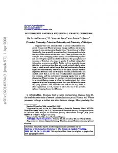
INS Uncertainty Ellipse

Picture Source: http://www.astrium-geo.com/en/65-satellite-imagery

Figure 1: Fusion of INS and Terrain Elevation Data Measurements

K ( f ; f 0 , M ) = M . log(

1 ) − log f 0 ( n) M

(13)

where n is the value of f0(x) at any given place; f0(x) is uniform. Given this, the following logic holds. CE is computed at the MAP, i.e. the strongest mode. The following can be deduced. • CE œ 0.75*i: The mode corresponding to MAP is very strong and other modes, if any, can be ignored. The error in this case can be approximated using variance of the corresponding mixture component. • 0.75*i > CE œ 0.60*i: KLD ≈ K(f; f0, 2) indicates two modes of similar strength; lower KLD indicates large variance for one mode with other modes being of lower strength. • 0.60*i > CE œ 0.40*i: KLD ≈ K(f; f0, 3) indicates presence of three modes of similar strength; lower KLD indicates large variance for one mode with other modes being of lower strength. • 0.40*i > CE œ 0.20*i: KLD ≈ K(f; f0, 4) indicates presence of four modes of similar strength; lower KLD indicates large variance for one mode with other modes being of lower strength. • CE < 0.20*i: Indicates very flat pdf; cannot be used meaningfully for any decision making. 5. Case Study: Terrain-Aided Navigation Use of Inertial Navigation System (INS) is well established in navigation systems; however, INS requires periodic resetting to bound error growth. GPS has many failure modes including active jamming [14]. For long-duration GPS outages, terrain-aided navigation (TAN) methods are appropriate [11,12,13]. TAN makes use of pre-recorded terrain contour map that is compared to measurements made during flight using a combination of Radio Altimeter (RADALT) that measures height above ground and Baro Altimeter that measures altitude above sea level [15]. Figure 1 depicts a sample case. Particles are initially distributed uniformly in this INS uncertainty zone. Weights are assigned to particles based on difference between stored and measured elevation data at that position. Particles are then resampled and the resulting posterior approximated as GMM. MAP is computed using (11) and (12), and INS uncertainty ellipse shrunk using the error estimation logic. Table 1. Parameter Values Parameter

Value

Parameter

Value

Terrain area

2kmX2km

Elevation Data and Noise

Resolution 1m, Accuracy 3m

Aircraft Speed

230m/s (0.8 Mach)

RADALT Sampling Frequency

100ms

GPS Update Rate

1 Hz

INS Position Drift

1 nautical mile/hour

RADALT Accuracy

±3 feet (1j) (At 200m above ground)

Baro Altimeter Accuracy

Baro errors assumed constant locally.

GPS Uncertainty

10m

Assumed INS Drift at Entry

250m

1003

Neeta Trivedi and N Balakrishnan / Procedia Computer Science 19 (2013) 998 – 1003

*: True x: Measured ♦: Estimated

*: True x: Measured ♦: Estimated

*: True x: Measured

*: True x: Meas red

Figure 2 (a): No Correction to INS Drift, (b): GPS Corrected Position, (c) TAN Corrected Positions, (d): With Variance Reduction

Figure 2 plots INS drift in the absence of any correction, position with GPS correction, estimates with TAN correction but without fusion, and position with TAN correction and fusion after error estimation. 6. Conclusions Many real-life problems lead to significantly multimodal posteriors; TAN is typical example. No state estimator is good for these situations. However, when pdfs from diverse sensor observations are fused, MAP estimate with different error indicators can help converge to true state faster. In this paper we have presented efficient MAP computation and novel error estimator for Bayes filter and its SMC approximation, with a case study on TAN. Simulation results and theoretical analysis demonstrate that use of the new error measures allow better state estimate and faster convergence.

References [1] [2] [3] [4] [5] [6] [7] [8] [9] [10] [11] [12] [13] [14] [15]

Mehlar RPS. Statistics Multisource-multitarget Information Fusion. Artech House, Norwood, MA: 2007 Sheng X, Hu Y-H, Ramanathan P. Distributed Particle Filter with GMM Approximation for Multiple Targets Localization and Tracking in Wireless Sensor Networks. Proc. IPSN 2005, 181-8, doi: 10.1109/IPSN.2005.1440923 Ma L-H, Zhang Y, Lu Z-M, and Li H. Research of Particle Filter Based on Immune Particle Swarm Optimization. J Info Tech 2013, 155-161, doi: 10.3923/itj.2013.155.161 Yan W, Torta E, Pol DVD, Meins N, Waber C, Cuijpers RH, Wermter S. Learning Robot Vision for Assisted Living. Chapter 15 – Robotic Vision: Technologies for the Machine, IGI Global, 257-80, doi: 10.4018/978-1-4666-2672-0.ch15 Zachariah D, Skog I, Jansson M, Händel P. Bayesian Estimation with Error Bounds. IEEE Signal Processing Letters 2012, 880-3, doi: 10.1109/LSP.2012.2224865 Kruecher C, Shapo B. Multitarget Detection and Tracking using Multisensor Passive Acoustic Data. IEEE J Ocean Engg 2011, 205-18, doi: 10.1109/JOE.2011.2118630 Ozdemir O, Niu R, Varshney PK, Drozd AL. Modified Bayesian Cramér-Rao Lower Bound for Nonlinear Tracking. Proc IEEE Intl Conf Acoustics, Speech and Signal Processing, May 2011, 3972-5, doi: 10.1109/ICASSP.2011.5947222 Dean AJ, Martini RD, Brennan SN. Terrain-based Road Vehicle Localization using Particle Filters. Intl J Vehicle Mechanics and Mobility 2011, 1209-23, doi: 10.1080/00423144.2010.493218 Carreira-Perpinan MA, Williams C. On the Number of Modes of a Gaussian Mixture. Informatics Research Report EDI-INFRR-0159, School of Informatics, Institute for Adaptive and Neural Computation, University of Edinburgh Carreira-Perpinan MA. Mode Finding for Mixture of Gaussian Distributions. IEEE Tr. Pattern Analysis and Machine Intelligence 2000, 1318-23 Bergman N. A Bayesian Approach to Terrain-aided Navigation II. Proc. SYSID 1997, 11th IFAC Symp System Identification Anonsen KB, Hallingstad O. Terrain-aided Underwater Navigation using Point Mass and Particle Filters. Proc. IEEE/ION Position, Location, and Navigation Symposium, Apr 2006, 1027-35, doi : 10.1109/PLANS.2006.1650705 Paul AS. Dual Kalman Filters for Autonomous Terrain-aided Navigation in Unknown Environments. Proc. IJCNN’05, Aug 2005, Vol 5, 2784-9, doi: 10.1109/IJCNN.2005.1556366 A Critical Review of the State-of-the-art in Autonomous Land Vehicle Systems and Technology, Sandia Report Number SAND2001-3685, Nov 2001 http://www.technologyreview.in/blog/mimssbits/26551/ last accessed 31-Dec-2012