State Feedback Tracking Control for Indirect Field-oriented Induction ...

International Journal of Automation and Computing

10(2), April 2013, 99-110 DOI: 10.1007/s11633-013-0702-4

State Feedback Tracking Control for Indirect Field-oriented Induction Motor Using Fuzzy Approach M. Allouche1 1

M. Chaabane

1

M. Souissi1

D. Mehdi2

F. Tadeo3

Laboratory of Sciences and Techniques of Automatic Control and Computer Engineering (Lab-STA), National School of Engineering of Sfax, University of Sfax, Postal Box 1173, 3038 Sfax, Tunisia 2 Laboratory of Computer and Automatic for System (LIAS), Higher School of Engineering of Poitiers (ESIP), University of Poitiers, 2 rue Pierre Brousse, Bt. B25-BP 633, 86022, Poitiers, France 3 Department of Systems Engineering, University of Valladolid, 47011 Valladolid, Spain

Abstract: This paper deals with the synthesis of fuzzy controller applied to the induction motor with a guaranteed model reference tracking performance. First, the Takagi-Sugeno (T-S) fuzzy model is used to approximate the nonlinear system in the synchronous d-q frame rotating with field-oriented control strategy. Then, a fuzzy state feedback controller is designed to reduce the tracking error by minimizing the disturbance level. The proposed controller is based on a T-S reference model in which the desired trajectory has been specified. The inaccessible rotor flux is estimated by a T-S fuzzy observer. The developed approach for the controller design is based on the synthesis of an augmented fuzzy model which regroups the model of induction machine, fuzzy observer, and reference model. The gains of the observer and controller are obtained by solving a set of linear matrix inequalities (LMIs). Finally, simulation and experimental results are given to show the performance of the observer-based tracking controller. Keywords:

1

Fuzzy tracking control, H∞ performance, feedback controller, linear matrix inequality (LMI), fuzzy observer.

Introduction

In the last two decades, the problem of tracking control for nonlinear systems has been dealt by several classic approaches, and many studies have been developed around this subject. However, there are a few works based on the Takgi-Sugeno (T-S) fuzzy model relating to the tracking control problem which have been studied for continuoustime systems[1−5] In our work, we are interested in the design of fuzzy observer-based tracking controller for an induction motor with H∞ performance. Induction motors are highly nonlinear systems, having uncertain time-varying parameters and subjected to unknown load disturbance. In addition, the rotor flux is inaccessible for state feedback control. Taking these difficulties into account, various control strategies, such as vector control method using proportional-integral (PI) controllers, input-output decoupling, control via geometric techniques, fuzzy adaptive control, and sliding mode control are proposed. A classical PI controller is a simple regulator used in the control of induction motor drives. However, the main drawback of this kind of controller is its sensitivity to the system-parameter variations and load changes[6, 7] . Thus, based on loop-shaping technique, a new control technique is proposed[8] to assure the disturbances rejection and lowering of tracking error. Wai and Chang[9] presented an adaptive observation system with an inverse rotor time-constant observer, based on a model reference adaptive system (MRAS) theory. The proposed adaptive system introduced in the control scheme guarantees the accurate estimation of the slip angular velocity, and preserves the decoupling control characteristic. In the last decade, many publications concerning the use of nonlinear inputoutput linearization techniques for the control of induction motors have been appeared. However, these approaches lose their performance when the motor parameters vary from Manuscript received February 21, 2011; revised June 3, 2012 This work was supported by AECID Projects (Nos. A/023792/09, A/030410/10 and AP/034911/11)

their nominal values and when a load torque is applied. As a result, Marino et al.[10, 11] proposed a direct adaptive controller for speed regulation, in which the motor model is input-output decoupled by a feedback-linearizing technique, while the load torque and rotor resistance are adapted in real time. The major inconvenience of this approach is the inability to ensure the asymptotic convergence of the system states and the estimated parameters. In the same context, a mixed H2 /H∞ optimized controller is used[12] to minimize the tracking error and to ensure the load torque disturbance rejection. A robust stability analysis method is presented via a parameter dependant Lyapunov function, in which the robust stability of the overall uncertain linearized closedloop system is tested. The sliding mode technique has been widely used in induction motor control and proved to have a small tracking error[13−15] , but the chattering phenomenon is inevitable, which degrades the performance of the system and may even lead to instability. Recently, fuzzy techniques have been widely and successfully used in induction motor modeling and control[16−18] . Among various fuzzy modeling methods, the well-known TS fuzzy model is considered as a popular and powerful tool in approximating a complex nonlinear system[19, 20] . The basic idea of this approach is to decompose the model of the nonlinear system into a series of linear models involving nonlinear weighting functions. The equivalent T-S fuzzy model describes the dynamic behavior of the system. The weighting functions checks the convex sum property. In this paper, the tracking problem for an induction motor is studied using the T-S fuzzy approach. First, a fuzzy augmented model is constructed by regrouping the T-S fuzzy model of the induction motor, a fuzzy observer, and the T-S reference model. Then, a fuzzy observer-based tracking controller is developed. The proposed T-S controller is dynamic and it has the characteristic to be adjustable through the insertion of the nonlinear weighting functions associated for every local controller. This property allows to adapt the global fuzzy controller inside the

100

International Journal of Automation and Computing 10(2), April 2013

polytope region [ismin , ismax ] × [ωmmin , ωmmax ] operating at various load torque and reference speed in order to improve the tracking performance. It also has the ability to achieve the favorable decoupling control and precision speed tracking property, even if the machine is subject to parametric variations. In addition, the tracking control design problem is parameterized in terms of a linear matrix inequality (LMI) problem which can be solved very efficiently using the convex optimization techniques. This paper is organized as follows. Section 2 presents an open-loop control strategy, which includes a physical model of the induction motor. Section 3 deals with the synthesis of a fuzzy control law with H∞ performance. To specify the desired trajectory, a T-S reference model is designed. The gains of the observer and controller are obtained by solving a set of LMIs. Section 4 gives the simulation and experimental results to highlight the effectiveness of the proposed control law. Section 5 gives conclusions on the main themes developed in this paper.

2

Open-loop control strategy

2.1

Physical model of induction motor

Under the assumptions of the linearity of the magnetic circuit, the electromagnetic dynamic model of the induction motor in the synchronous d-q reference frame can be described as x(t) ˙ = f (x(t)) + g(x(t))u(t) + w(t)

(1)





where

      f (x(t)) =         g(x(t)) = 

Ks Ψrd + Ks np ωm Ψrq τr Ks Ψrq −ωs isd − γisq − Ks np ωm Ψrd + τr 1 M isd − Ψrd + (ωs − np ωm )Ψrq τr τr 1 M isq − (ωs − np ωm )Ψrd − Ψrq τr τr np M f (Ψrd isq − Ψrq isd ) − ωm JLr J T 1 0 0 0 0  σLs  1 0 0 0 0 σLs

−γisd + ωs isq +

u(t) = [usd usq ]T x(t) = [isd isq Ψrd Ψrq ωm ]T ·

Cr w(t) = 0 0 0 0 − J ¶ µ 1 1−σ γ= + στs στr Ks = τr =

M σLs Lr Lr Rr

¸T

           

τs =

Ls Rs

σ =1−

M2 Ls L r

where ωm is the rotor speed, ωs is the electrical speed of stator, (Ψrd , Ψrq ) are the rotor fluxes, (isd , isq ) are the stator currents, and (usd , usq ) are the stator voltages. The load torque Cr is considered as an unknown disturbance. The motor parameters are moment of inertia J, rotor and stator resistances (Rs , Rr ), rotor and stator inductances (Ls , Lr ), mutual inductance M, friction coefficient f, and number of pole pairs np .

2.2

Open-loop control

In this section, the structure of the open-loop control strategy is explored, which will be modified in the next section to design the closed-loop T-S reference model. If we replace the state variables of the motor [isd isq Ψrd Ψrq ωm ]T by the corresponding reference signals [isdc isqc Ψrdc 0 ωmc ]T in (1), we obtain[21]                

Ks 1 d isdc = −γisdc + ωs isqc + Ψrdc + usdc dt τr σLs 1 d isqc = −ωs isdc − γisqc − Ks np ωmc Ψrdc + usqc dt σLs M isqc 0 = −(ωs − np ωmc )Ψrdc +  τr     d M 1   Ψrdc = isdc − Ψrdc   dt τ τ  r r    np M f 1  d  ωmc = (Ψrdc isqc ) − ωmc − Cr . dt JLr J J (2) The last two equalities in (2) lead to the open-loop reference stator currents as  τr d Ψrdc    isdc = M + M dt Ψrdc ¶ µ (3) f d Cr JLr   + ωmc + ωmc .  isqc = np M Ψrdc J J dt According to (2), the electrical speed reference of the stator is given as ωsc = np ωmc +

M isqc . τr Ψrdc

(4)

From the first two equalities in (2), we obtain the expression of the open-loop control as  ¶ µ Ks d   isdc + γisdc − ωsc isqc − Ψrdc  usdc = σLs τr µ dt ¶ d   isqc + γisqc + ωsc isdc + Ks np ωmc Ψrdc .  usqc = σLs dt (5)

3

Fuzzy observer-based tracking control

The nonlinear model (1), described in the synchronous dq frame, is transformed into an equivalent T-S fuzzy model using the linear sector transformation[22] . The global linear fuzzy model is composed of a set of linear models which are

M. Allouche et al. / State Feedback Tracking Control for Indirect Field-oriented Induction Motor Using Fuzzy Approach

interpolated by membership functions. The synthesis of a fuzzy controller requires the construction of the augmented fuzzy model, which regroups the T-S fuzzy model of the induction motor, the fuzzy observer, and the reference model. The premise variables are assumed to be measurable.

3.1

where the membership functions can be written as  zk (t) − zk min    Fk,min (zk (t)) = z k max − zk min  z − zk (t)   Fk,max (zk (t)) = k max . zk max − zk min

T-S fuzzy model of induction motor

The field-oriented strategy when is implemented relative to the synchronously rotating frame of reference, allows for an independent control of the torque and of the rotor flux. In this case, the dynamics of the induction motor is similar to the separately excited DC motor. In this condition, the rotor flux vector (Ψrd , Ψrq ) is aligned to the d-axis, and the results can be obtained as ½ Ψrd = Ψrdc (6) Ψrq = 0.

(11)

The fuzzy model is described by fuzzy If-Then rules and will be employed here to deal with the control design problem for the induction motor. The i-th rule of the fuzzy model for the nonlinear system is described in the following form: Rule Ri : If (z1 (t) is F1,l ) and (z2 (t) is F2,f ) and (z3 (t) is F3,h ) Then x(t) ˙ = Ai x(t) + Bu(t) + w(t) with l, f, h ∈ {min, max}, and i = 1, 2, · · · , 8. The global fuzzy model is inferred as

To assure condition (6), the electrical speed of the stator in the rotating synchronous d-q frame must be chosen as M ω s = np ω m + isq . τr Ψrdc

101

x(t) ˙ =

8 X

hi (z(t))(Ai x(t) + Bu(t) + w(t))

(12)

λi (z(t)) 8 P λi (z(t))

(13)

i=1

(7) with

If we replace the electrical speed of the stator (7) in the physical model (1), the nonlinear model of the induction motor can be written as the state space form: ½ x(t) ˙ = Ax(t) + Bu(t) + w(t) (8) y = Cx(t) + v(t)

hi (z(t)) =

i=1

λi (z(t)) =

where

3 Y

Fik (zk (t))

(14)

k=1



−γ

   −ωs    M  A(x(t)) =  τr    0    0

Ks τr −Ks np ωm

ωs −γ 0

0



1  σLs B= 0 

1 C= 0 0

0 1 0

0 1 σLs 0 0 0

1 τr M − isq τr Ψrdc np M isq JLr T 0 0 0   0 0 0 −

M τr

0 0 0

K s np ω m Ks τr M isq τr Ψrdc 1 − τr np M − isd JLr



0 0 0 0 f − J

             

8 X

and v(t) represents the measurement noise. Considering the sector of nonlinearities of the terms zk (t) = xk (t) ∈ [zk min , zk max ] of the matrix A(x(t)) with k = 1, 2, 3 yields    z1 (t) = isd (t) z2 (t) = isq (t) (9)   z3 (t) = ωm (t). Thus, we can transform the nonlinear terms into the following shape: (10)

hi (z(t)) = 1.

i=1

where hi (z(t)) is regarded as the normalized weight of each model rule, and Fik (z(t)) is the grade of membership of zk (t) in Fik .

3.2

 0 0  1

zk (t) = Fk,min (zk ) × zk max + Fk,max (zk ) × zk min

hi (z(t)) > 0

T-S reference model

The open-loop response of the induction motor defined by the control input (5) is characterized by an important overshoot of the d-axis rotor flux (see Appendix D). In order to improve the transient performance of the system, we consider a nonlinear reference model via a T-S fuzzy approach. The designed T-S reference model is a piecewise interpolation of several linear models through membership functions. The dynamics of the closed-loop system is modified through the insertion of positive parameters Ki and KΨ in the T-S reference model, which has the desired dynamics behavior. Therefore, we define the new control input vector as   u0 = usdc + Ki σLs (isdc − isdr ) + σM KΨ (Ψrdc − Ψrdr ) sdc τr  0 usqc = usqc + Ki σLs (isqc − isqr ). (15) Consider the reference state of the closed-loop system xr (t) = [isdr isqr Ψrdr Ψrqr ωmr ]T . It is the desired trajectory for x(t) to follow.

102


The above equality (15) can be written as    d  i + (γ + K )i − ω i  i sc sqc sdc sdc   dt    − µ ¶  u0sdc = σLs      M K − L K Ψ s s   + Ψrdc   τ L  r s   {z } |    usdr   ¶ µ    σM KΨ   Ψrdr Ki σLs isdr − τr          d   i +(γ + K )i +ω i  sqc i sqc sc sdc  −Ki σLs isqr  u0sqc = σLs  dt     +Ks np wmc Ψrdc    | {z }    usqr    (16) This is equivalent to  ¶ µ   u0 = usdr − Ki σLs isdr − σM KΨ Ψrdr sdc τr   u0 = u − K σL i . sqr i s sqr sqc

   −ωsr    M Ar =   τr    0   0

ωsr

K2

−K1

−Ks np ωmr 1 τr M − isqr τr Ψrdc np M isqr JLr

0

−

M τr 0

K1 = (γ + Ki ), K2 = (

Ks np ωmr Ks τr M isqr τr Ψrdc 1 − τr np M − isdr JLr

0



      0 ,    0   f  − J 0

Ks M KΨ − ), and ωsr = np ωmr + τr Ls τr

M isqr . r(t) is a bounded input given as τr Ψrdc · ¸ Ur r(t) = [B I] w(t) where Ur =

£

usdr

usqr

¤T

8 X

hrj (zr (t))Arj xr (t) + r(t)

(20)

λrj (zr (t)) 8 P λrj (zr (t))

(21)

j=1

with hrj (z(t)) =

j=1

λrj (zr (t)) =

3 Y

Njk (zrk (t)).

(22)

k=1

P For all hrj (zr (t)) > 0, and 8j=1 hrj (zr (t)) = 1. hrj (zr (t)) is regarded as the normalized weight of each reference rule. Njk (zr (t)) is the grade of membership of zrk (t) in Njk .

er (t) = x(t) − xr (t).

(17)

where −K1

x˙ r (t) =

Define the tracking error as

Given the new control input (17) in the physical model (1), and replacing the state x(t) by xr (t), the nonlinear model of the induction motor leads to the state space reference model: x˙ r (t) = Ar xr (t) + r(t) (18) 

where N1,l , N2,f and N3,h are the fuzzy sets which have the same structure as (11). The global fuzzy reference model is inferred as

.

The reference model (18) is nonlinear and can be described via a T-S fuzzy model. Rule Rj : If (zr1 (t) is N1,l ) and (zr2 (t) is N2,f ) and (zr3 (t) is N3,h ) Then x˙ r (t) = Arj xr (t) + r(t) with l, f, h ∈ {min, max}, i = 1, 2, · · · , 8, zr1 (t), zr2 (t) and zr3 (t) are the measurable premise variables defined as    zr1 (t) = isdr (t) zr2 (t) = isqr (t) (19)   zr3 (t) = ωmr (t)

(23)

Then, the objective is to design a T-S fuzzy model-based controller which stabilizes the closed-loop fuzzy system and achieves the H∞ tracking performance related to the tracking error er (t) given by Z tf Z tf 2 ¯ eT φ¯T (t)φ(t)dt (24) r (t) Q er (t) dt 6 ρ 0

0

where φ¯ = [v(t) w(t) r(t)]T for all reference input r(t), external disturbance w(t), and measurement noise v(t). tf represents the terminal time of control, Q is a positive definite weighting matrix, and ρ a prescribed attenuation level.

3.3

Tracking control design

To design an observer-based tracking controller, a new parallel distributed compensation (PDC) controller is proposed. The main difference from the ordinary PDC controller described in [23] is to have a term of xr (t) in the feedback control law. Then, the new PDC fuzzy controller is designed as[24] Sub-controller A rule Ri : If (z1 (t) is F1,l ) and (z2 (t) is F2,f ) and (z3 (t) is F3,h ) Then uA (t) = Ki x ˆ(t) for i = 1, 2, · · · , 8. Sub-controller B rule Rj : If (zr1 (t) is N1,l ) and (zr2 (t is N2,f ) and (zr3 (t) is N3,h ) Then uB (t) = −Kj xr (t) for j = 1, 2, · · · , 8. Hence, the overall fuzzy controller is given by u(t) = uA (t) + uB (t) u(t) =

8 X i=1

hi (z(t)) Ki x ˆ(t) −

8 X

(25)

hrj (zr (t)) Kj xr (t). (26)

j=1

However, the fuzzy tracking control law (26) requires that all state variables are available. In this condition, a fuzzy observer of Luenberger type is constructed to estimate the immeasurable states of the rotor flux. According to the fuzzy model (12), the fuzzy observer is given as If (z1 (t) is F1,l ) and (z2 (t) is F2,f ) and (z3 (t) is F3,h )

M. Allouche et al. / State Feedback Tracking Control for Indirect Field-oriented Induction Motor Using Fuzzy Approach

Then x ˆ˙ (t) = (Ai x ˆ(t) + Bu(t) + Li (y(t) − yˆ(t))) where Li is the gain of the observer. The overall fuzzy observer is represented as  8 X  x ˆ˙ (t) = hi (z(t))(Ai x ˆ(t) + Bu(t) + Li (y(t) − yˆ(t))) i=1   yˆ(t) = C x ˆ(t). (27) Define the observation error e(t) = x(t) − x ˆ(t).

(28)

From systems (12), (27) and (28), we can obtain the error dynamics as e(t) ˙ =

8 X

103

¯ φ(t). The main result of fuzzy observer-based tracking control for the T-S fuzzy model of the induction motor is summarised in the following theorem: Theorem 1. If there exists a symmetric and positive definite matrix P¯ = P¯ T > 0 and a prescribed positive constant ρ2 such that 1 ¯ ¯ ¯T ¯ ¯T ¯ ¯¯ ¯ G ij P + P Gij + 2 P Fi Fi P + Q < 0 ρ

(32)

then the performance of H∞ tracking control for the prescribed ρ2 is guaranteed, and the quadratic stability for the closed-loop system is assured. Proof. Consider the Lyapunov function V (¯ x(t)) = x ¯T (t)P¯ x ¯(t) where P¯ = P¯ T > 0. The time derivative of V (¯ x(t)) is

hi (z(t)) [(Ai − Li C)e(t) − Li v(t)] + w(t). (29) V˙ (¯ x(t)) = x ¯˙ T (t)P¯ x ¯(t) + x ¯T (t)P¯ x ¯˙ (t)+

i=1

The augmented system composed of equalities (12), (20) and (29) can be expressed as

8 X 8 X

¯T ¯ ¯¯ hi (z(t))hj (zr (t))[¯ xT (t) (G ¯(t)+ ij P + P Gij ) x

i=1 j=1

x ¯˙ (t) =

8 X 8 X

£ ¤ ¯ ¯ ij x hi (z(t))hj (zr (t)) G ¯(t) + F¯i φ(t) (30)

i=1 j=1



 e(t) x ¯(t) =  x(t)  xr (t)

Gij

Ai − Li C =  −BKi 0 

F¯ =  

−Li 0 0

I I 0

X T Y + Y T X 6 ρ2 X T X +  0 −BKj  Arj

0 Ai + BKi 0 0 0  I

1 T Y Y ρ2

where ρ is a real value which is assumed to be positive. Applying the statement of Lemma to the term ¯ φ¯T (t) F¯iT P¯ x ¯(t) + x ¯T (t)P¯ F¯i φ(t)

 we obtain

¯ 6 φ¯T (t) F¯iT P¯ x ¯(t) + x ¯T (t)P¯ F¯i φ(t) 1 T ¯ ¯ ¯T ¯ ¯ x ¯ (t)P Fi Fi P x ¯(t) + ρ2 φ¯T (t) φ(t). ρ2



v(t) ¯ =  w(t)  . φ(t) r(t) Hence, the H∞ tracking performance in (24) can be modified as follows, if the initial condition is also considered[2, 25, 26] : Z tf (x(t) − xr (t))T Q (x(t) − xr (t)) dt = 0 Z tf ¯x x ¯T (t) Q ¯(t) dt 6 0 Z tf ¯ φ¯T (t) dt φ(t) (31) x ¯T (0)P¯ x ¯(0) + ρ2 0

where

(33)

¤ Lemma 1. For any matrices X and Y with appropriate dimensions, the following property holds:

where



¯ φ¯T (t) F¯iT P¯ x ¯(t) + x ¯T (t)P¯ F¯i φ(t)].

(34)

Substituting (34) into (33) yields V˙ (¯ x(t)) 6 h

8 X 8 X

hi (z(t))hj (zr (t))¯ xT (t)×

i=1 j=1

¯T ¯ ¯¯ G ij P + P Gij

i x ¯(t)+

1 T ¯ ¯ ¯T ¯ ¯ 6 x ¯ (t)P Fi Fi P x ¯(t) + ρ2 φ¯T (t) φ(t) ρ2 8 X 8 X hi (z(t))hj (zr (t))¯ xT (t)× i=1 j=1



0 ¯= 0 Q 0

0 Q −Q



0 −Q  Q

and P¯ is a symmetric positive definite weighting matrix. Now, the objective is to determine the controller0 s and observer0 s gains Ki and Li for the augmented model (30) with the guaranteed H∞ tracking performance (24) for all

1 ¯ ¯ ¯T ¯ ¯ ¯¯ ¯T [G x(t)+ ij P + P Gij + 2 P Fi Fi P ]¯ ρ ¯ ρ2 φ¯T (t) φ(t). From (32), we get ¯ ¯x V˙ (¯ x(t)) 6 −¯ xT (t) Q ¯(t) + ρ2 φ¯T (t) φ(t).

(35)

104


where

Integrating (35) from t = 0 to t = tf yields V (tf ) − V (0) 6 Z tf Z tf ¯ dt 6 ¯x − x ¯T (t) Q ¯(t) dt + ρ2 φ¯T (t) φ(t) 0 0 Z tf Z tf ¯ dt. − er (t)T Q er (t) dt + ρ2 φ¯T (t) φ(t) 0

T T D11 = AT i P1 + P1 Ai − Ci Zi − Zi Ci 1 D14 = −(Bi Ki )T P2 + 2 P1 P2 ρ

D44 = (Ai + BKi )T P2 + P2 (Ai + BKi ) + (36)

0

D45 = −P2 (BKj ) − Q D55 = AT rj P3 + P3 Arj + Q.

This is equivalent to Z

tf

1 P 2 P2 + Q ρ2 (41)

T

er (t) Q er (t) dt 6

0

Z er (0)T Q er (0) + ρ2

tf

¯ dt. φ¯T (t) φ(t)

(37)

0

As a result, the H∞ tracking control performance is achieved with a prescribed attenuation level ρ. It is noted that Theorem 1 gives the sufficient condition of ensuring the stability of the augmented fuzzy system (30) and achieving the tracking performance (24). However, it does not give the methods of obtaining the solution of the common positive matrices, the gains of fuzzy controller and fuzzy observer. Inequality (32) presents bilinear matrix inequality (BMI) conditions. For this reason, we propose a method that consists of solving these BMI0 s in two stages, such that every stage is considered as a standard LMI[2, 25] . To facilitate the resolution, the matrix variable P¯ is chosen diagonal with respect to appropriate matrix blocks: P¯ = diag{ P1

P2

P3 }.

(38)

Using LMI tools, there are several parameters that should be determined from (40). There are no effective algorithms for solving them simultaneously. However, we can solve them by the following two-step procedure. First, we can find P2 and Ki from the diagonal blocks D44 , then P1 , P3 and Li from the inequality (40). Indeed, after congruence of (40) with diag{I, I, I, P2−1 , I, I}, considering the change of variable N2 = P2−1 , Yi = Ki N2 , and using the Schur0 s complement, D44 is equivalent to the following LMI:   1 T T N N 2 Ai + Ai N2 + BYi + (BYi ) + 2 I 2   < 0. ρ N2 −Q−1 (42) The parameters P2 = N2−1 and Ki = Yi N2−1 are obtained by solving the LMIs in (41). In the second step, by substituting P2 and Ki into inequality (40), the last condition becomes a standard LMI, and we can easily solve P1 , P3 and the observer0 s gains Li .

4

Simulation and experimental results

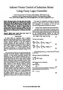
The proposed fuzzy tracking control law has first been tested in simulation as shown in Fig. 1.

By substituting (38) into (32), we obtain 

II11  II21 0

II12 II22 II32

 0 II23  < 0 II33

(39)

where 1 II11 = (Ai − Li Ci )T P1 + P1 (Ai − Li C) + 2 P1 (Li LT i + I)P1 ρ 1 T II12 = II21 = −(BKi )T P2 + 2 P1 P2 ρ 1 II22 = (Ai + BKi )T P2 + P2 (A + Bi Ki ) + 2 P2 P2 + Q ρ T II23 = II32 = −P2 (BKj ) − Q 1 T II33 = Arj P3 + P3 Arj + 2 P3 P3 + Q. ρ We consider the change of variable Zi = P1 Li . Using the Schur complement, inequality (39) is equivalent to 

D11  P1  T  Zi  T  D14   0 0

P1 −ρ2 I 0 0 0 0

Zi 0 −ρ2 I 0 0 0

D14 0 0 D44 T D45 0

0 0 0 D45 D55 P3

0 0 0 0 P3 −ρ2 I

    