X Robust Shaping Indirect Field Oriented Control for Induction Motor

Robust Shaping Indirect Field Oriented Control for Induction Motor

59

X4 Robust Shaping Indirect Field Oriented Control for Induction Motor M. Boukhnifer, C. Larouci and A. Chaibet Laboratoire Commande et Systèmes, ESTACA, 34-36 rue Victor Hugo, 92 300 Levallois-Perret, France {mboukhnifer, clarouci, achaibet}@estaca.fr

1. Introduction Over the past years, thanks to the systematic use of digital microprocessors in industry, we have seen a very significant development in the regulation controls of the asynchronous machine. The latter is widely used in industry for its diversity of use and its ability to withstand great variations in its nominal regime. Currently, several types of control are proposed. Nonlinear controls such as linearization input-output (Benchaib & Edwards, 2000) (Chan et al., 1990) (De Luca & Ulivi, 1989) (Marina & Valigi, 1991), the controls resulting from the theory of passivity (Nicklasson et al., 1997) (Gokdere, 1996) which generally require the measurement of all system states (currents and flux). As the flux of the motor cannot be measured, a great part of the literature is devoted to the control problem coupled with a nonlinear flux observer (Kanellakopoulos et al., 1992). Other controls using only the exit returns (rotor speed and stator currents) were developed resulting in controls of the passive type (Abdel Fattah & Loparo, 2003), other controls using the technique of backstepping or the techniques derived from the orientation of the flux field (Peresada et al., 1999) (Barambones et al., 2003). The parameters of such controls must be selected in order to ensure total stability for a given nominal running and nominal values of the parameters. Thus, different robust controls with parameter uncertainties, such as the discontinuous or adaptive controls, were developed (Marina et al., 1998). These techniques adapt the controls to the variations of resistances and the load couple. A control which is very common in industry is the indirect field oriented control (FOC) based on the orientation of the field of rotor flux. This control allows the decoupling of speed and flux, and we obtain linear differential equations similar to the D.C. machine. The regulation is carried out finally by simple controller PI (cf Fig. 1). However, the decoupling observed is only asymptotic. The behaviour of the transient regime and the total stability of the system remain a major problem. In addition, the modifications of parameters such as rotor resistance or resistive torque deteriorate the quality of decoupling. In this paper, we propose a diagram of H  regulation, linked to the field oriented control allowing a correct transient regime and good robustness against parameter variation to be

60

Mechatronic Systems, Simulation, Modelling and Control

ensured. This Paper is divided into several parts: The first one describes the model of the asynchronous machine, using the assumptions of Park. In the second part, we present the field oriented control principles, as well as regulation simulations, using PI. The third part is devoted to the problems of the H  control and the loop shaping design procedure approach originally proposed in (McFarlane et al., 1988) and further developed in (McFarlane & Glover, 1988) and (McFarlane & Glover, 1989) which incorporates the characteristics of both loop shaping and H  design. Specifically, we make use of the socalled normalized coprime factor H  robust stabilization problem which has been solved in (Glover & McFarlane, 1988) (Glover & McFarlane, 1989) and is equivalent to the gap metric robustness optimization as in (McFarlane & Glover, 1992). The design technique has two main stages: 1) loop shaping is used to shape the nominal plant singular values to give desired open-loop properties at frequencies of high and low loop gain; 2) the normalized coprime factor H  problem mentioned above is used to robustly stabilize this shaped plant. Finally, the last part shows how to integrate the loop shaping design procedure into the field oriented control with the Luenberger observer and proposes simulations results.

2. Mathematical model of asynchronous machine We use some simplifying assumptions and Park transformation. The stator currents ( I ds , I qs ) , the rotor flux ( dr , qr ) and the rotation speed wm are considered as state variables. The model of the asynchronous machine in the reference axes d, q related to the rotating field is given in the form: .

X  f ( x)  BU

(1)

X  ( I ds , I qs , dr ,qr , wm )T is the state vector. U  (vds , vqs )T is the control vector.    L2  L  dI ds 1   m m     Rs  Rr 2 I ds  s LsI qs   T L dt L   L  r r s   r      L2   dI qs  1     L  I   R  R m  I  p s s ds  s r 2  qs m L   dt L s  r     d L  dr  m I  1   w   dt dr gl qr T ds T r r   d L 1  qr m  dt  T I qs  wgl  dr  T  qr  r r  d 1  m   dt  J  Cem  Cr  k f m   

 L m  v  qr ds  m L  r   L L m   m  v  qr qs  dr T L L  r r r  

dr

 p

(2)


wgl  ws  w, ws 

d , w  pwm dt

Cem  p ( I qsdr  I ds qr ),  r   dr2   qr2

  1

61

(3)

Lm L , Tr  r Ls Lr Rr

Where J is the moment of inertia. L r , L s and Lm are respectively rotor inductance, stator inductance and mutual inductance. R r and R s are respectively the resistance of the rotor and of the stator , P is the number of pole pairs of the machine, k f is the friction coefficient and  is Blondel’s dispersion coefficient .

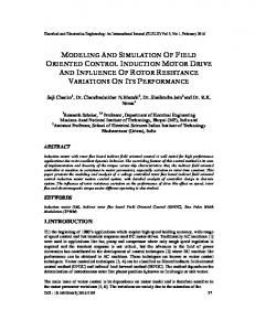
3. Indirect field oriented control The aims of this method of frequency control (Slipway Frequency Control) consist in not using the flux rotor amplitude but simply its position calculated according to the reference variables (Peresada et al., 1999) (Blaschke, 1972). This method does not use a flux sensor (physical sensor or dynamic model) but needs the rotor speed sensor. Fig.1 shows an example of an applied indirect field control with a type PI regulation on the asynchronous machine fed by an inverter controlled by the triangulo-sinusoidal strategy with four bipolar carriers. 3.1 Field oriented control The FOC (Field Oriented Control) is an arithmetic block which has two inputs (  r* and Cem* ) and generates the five variables of the inverter (Vds* ,Vqs* , ws* , I *ds , I *qs ) . It is defined by leading the static regime for which the rotor flux and the electromagnetic couple are maintained constant equal to their reference values. If we do not take into account the variations of the direct currents and the squaring component, the equations of this block are deduced in the following way:  * i ds*  r  Lm  L C*  i qs*  r em*  pLm r   L R i*   *    m r qs m  s Lr  r* v *  R i *   *L i * s ds s s qs  ds  v qs*  R s i qs*   s* Ls i ds*

(4)

This method consists to control the direct component I ds and the squaring I qs stator current in order to obtain the electromagnetic couple and the flux desired in the machine.

62


Inverter *

va

m  r*

m

* Cem

*

-

k

p

*

vb

MAS

* c

v

 s*

Park -1 vqs

*

vds

*

FOC

 k i S

m

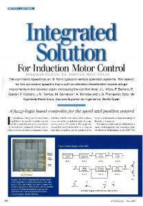
Fig. 1. Indirect field control of asynchronous machine 3.2 Simulation of field oriented control The best-known inverters up to now are the two level inverters. However, some applications such as electric traction require three-phase asynchronous variators functioning at very high power and/or speeds. These two level inverters are limited in tension (1,4kV) and power (1MVA). To increase power and tension, we use a multilevel inverter. In our work, the multilevel inverter used is controlled by the triangulo-sinusoidal strategy with four bipolar carriers (Boukhnifer, 2007). Fig.2 shows the results of the indirect field control of an asynchronous machine fed by this inverter. The decoupling is maintained and the speed follows the reference very well and is not affected by the application of a resistive torque. In the next section, we will explain briefly the principles of the H  control and how it can be integrated into the indirect field control.

4. Robust control 4.1 H∞ Control For given P(s) and  >0, the H  standard problem is to find K(s) which: - Stabilize the loop system in Fig. 3 internally. - Maintain the norm FL ( P, K )    with FL(P, K) defined as the transfer function of exits Z according to entries W. 4.2 H  Coprime factorization approach An approach was developed by McFarlane and Glover (McFarlane & Glover, 1988) (McFarlane & Glover, 1989) starting from the concept of the coprime factorization of a transfer matrix. This approach presents an interesting properties and its implementation uses traditional notions of automatics.


63

W

FL(p ,K)

Z P(s)

U

K

Y

Fig. 3. Problem H  standard

t(s)

t(s)

t(s)

t(s)

t(s)

t(s)

Fig. 2. Simulation of the indirect field control of asynchronous machine 4.3 Robust controller design using normalized coprime factor We define the nominal model of the system to be controlled from the coprime factors on the left: G  M~ 1  N~ . Then the uncertainties of the model are taken into consideration so that (see Fig. 4) ~ ~ ~ G  ( M   M ) 1  ( N   N )

~ G

K

N

~ N

Fig. 4. Coprime factor stabilization problem

M1 ~ M 1

(5)

64


~ where G is a left coprime factorization (LCF) of G, and  M ,  N are unknown and stable transfer functions representing the uncertainty. We can then define a family of models as follows:

~

~

~

  G  ( M   M )  ( N   N ) : ( M  N )    max 

(6)

Where  max represents the margin of maximum stability. The robust stability problem is thus to find the greatest value of    max , so that all the models belonging to   can be stabilized by the same corrector K. The problem of robust stability H  amounts to finding

 min and K(s) stabilizing G(s) so that: I  1    ( I  K  G ) 1 ( I G )   min  K  max  

(7)

However, McFarlane and Glover (McFarlane & Glover, 1992) showed that the minimal value of  is given by: 1  min   max  1  sup ( XY )

(8)

where sup indicates the greatest eigenvalue of XY, moreover for any   max , a controller stabilizing all the models belonging to   is given by: where A, B and C are state matrices of the system defined by the function G and X, Y are the positive definite matrices and the solution of the Ricatti equation :

AT X  XA  XB T BX  C T C  0

(9)

AY  YAT  YC T CY  BB T  0

4.4 Loop-shaping design procedure Contrary to the approach of Glover-Doyle, no weight function can be introduced into the problem. The adjustment of the performances is obtained by affecting an open modelling (loop-shaping) process before calculating the corrector. The design procedure is as follows: G(s) W1 W2 Ga(s) reference

K (0)  W 2 (0)

W1

G(s)

W2

K (s) Fig. 5. The loop-shaping design procedure We add to the matrix G(s) of the system to be controlled a pre-compensator W1 and/or a post-compensator W2, the singular values of the nominal plant are shaped to give a desired open-loop shape. The nominal plant G(s) and shaping functions W1 and W2 are combined in


65

order to improve the performances of the system so that Ga  W1GW2 (see Fig.5). In the monovariable case, this step is carried out by controlling the gain and the phase of Ga ( jw) in the Bode plan. From coprime factorizations of Ga ( s ) , we apply the previous results to calculate  max , and then synthesise a stabilizing controller K ensuring a value of slightly lower than  max : I     ( I  K  W2  G  W1 ) 1 ( I W2  G  W1 ) K

  

1 

(10)

The final feedback controller is obtained by combining the H controller K with the shaping functions W1 and W2 so that Ga(s) = W1GW2. (See Fig.5).

5. Robust control of the asynchronous machine When the reference is directed we have  dr   r and  qr  0 . In this case, the expression of the electromagnetic couple can be written in the form: C em  kids iqs

,

k

p Lr

(11)

This equation simplifies the model of the asynchronous machine as follows:  dI ds L L R 1  (( Rs  ( m ) 2 Rr )ids  Ls s iqs  m 2 r r  vds )  dt L L  Lr s r   dI qs Lm 2 Lm 1   r m  vqs ) (Ls s ids  ( Rs  ( ) Rr )iqs  Lr Lr  dt Ls  d R  r Lm Rr  ids  r r  Lr Lr  dt  d p 2 Lm f p  m  iqsr  m  Cr Lr J J J  dt      Lm Rr i m qs  s Lr r

(12)

By using the transform of Laplace, we can write that: r 

lm p  lm C em  I ds , C em   r  I qs ,   lr lr J s  kf 1  s rr

(13)

The equation (13) shows that we can act independently on rotor flux and the electromagnetic couple by means of components I ds and I qs respectively of the stator current. The goal consists in controlling the direct component I ds and in squaring component I qs of the stator current in order to obtain the electromagnetic couple and the flux desired in the machine. We can represent our system by combining equations (3) and (13) in two sub-systems with the transfer functions described below, See (Boukhnifer, 2007) for details:

66


G flux 

1 Tr s  1 Tr

1J skf J

Gvitesse 

(14)

In order to ensure a high gain in low frequencies and a low gain in high frequencies, we add the weight functions for flux and speed respectively so that . W 

2  ( s  5) s

W 

2.5  ( s  2) s

(15)

5.1 Loop shaping controller The calculation of the flux controller by MATLAB® software gives: 0.8140  s  6.7347 s  5.4817

(16)

 max  0.7756

The calculation of the speed controller by MATLAB® software gives: 1.0208  s  1.9587 s  1.9994

 max  0.6998

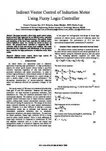
K2(s)

Inverter * a

v

 r* K 2(0)

+

-

* m

K1(0)

* Cem

+

w1(s)

-

MAS

*

vc

 s*

Park -1

W2(s) vqs



*

vb

*

(17)

vds

*

FOC m

K1(s)

Fig. 6. Robust control of asynchronous motor 5.2 Simulation of the robust control To illustrate the performances of the H∞ control, we simulated a no-load start with application of the load (nominal load Cr=10Nm) at t1 = 1.5Sec to t2 = 2.5Sec. Then the machine is subjected to an inversion of the instruction between 100 rad/sec at t3=3Sec (Fig.7). The speed regulation presents better performances with respect to the pursuit and the rejection of the disturbances. We note that the current is limited to acceptable maximum values. The decoupling is maintained and the speed follows the reference well and is not affected by the application of a resistive torque.

6. Luenberger observer We apply the Luenberger observer method for the estimation of the rotor flux components (Orlawska-Kowalska, 1989). The model of the reference machine linked to the stator field is


67

linear in the electromagnetic states. The two stator current components are measurable. We will consider them as outputs of the model: x  Ax  Bu (18) y  Cx with:  u   vs  u   1    ,  u 2   vs 

 x1   is       y1   is   x   i s  y      , x        x  y 2   is   3   r   x     4   r 

(19)

and:       A  Lm T  r  0  

0

k Tr



 pk

0 Lm Tr



1 Tr

p

 pk   1   k   Ls   Tr  , B 0   p   0   0 1    Tr 

 0   1   1 0 0 0  , c   Ls   0 1 0 0 0  0 

(20)

Fig. 7. Simulation results of robust control of asynchronous motor For the observation of the states x3  r and x4   r we use the following Luenberger observer:

zˆ  Fzˆ  ky  Hu

(21)

The dimensions of the vectors and matrices which appeared in this relation are:

z (3,1), F (2,2), k (2,2), H (2,2).

(22)

68


Vector Z is related to the initial state vector x by the transformation matrix T: Z=Tx

(23)

To determine the relations between the matrices of system A,B and C and the matrices of the observer F, K and H, the equation of error is calculated (e  zˆ  Tx) :

e  zˆ  Tx  Fzˆ  ky  Hu  T Ax  T Bu  Fzˆ  k Cx  Hu  T Ax  T Bu

(24)

 F (e  Tx)  k Cx  Hu  T Ax  T Bu  Fe  ( FT  k C  T A) x  ( H  T B)u To give the equation of error the form:

e  Fe

(25)

We must check the relation: TA  FT  KC H  TB

(26)

The error dynamics (25) is described by the eigenvalue of the state matrix of observer F. We impose to this matrix the following form:

F  diag (1 ,  2 )

(27)

In order to stabilize the error dynamics, λ 1 and λ2 must be negative. With this choice of F, the explicit equations of the observer are given by:

z1  1 z1  k11 y1  k12 y 2  h11u1  h12 u 2 z 2  2 z 2  k 21 y1  k 22 y 2  h21u1  h22 u 2

(28)

We impose to the transformation matrix T the following form: t T   11  t 21

t12 t 22

1 0  0 1 

The elements of the T, K matrix and H are obtained from the equations (25):

(29)


t11  t11 

 r2  1 r  p 2 2 k  r2  p 2  2 



1 p

k  r2  p 2 2

t12 



k11  (  1 ).t11  Lm r k21  (  1 ).t21 h11  h21 

t11

Ls t 21

Ls

h12  h22 

1 p k  r2  p 2  2



69



 2     p 22 t22  r 21 r 2 2 k  r  p   k12  (  2 ).t12 k22  (  2 ).t11  Lm r

(30)

t12

Ls t22

Ls

From equation (23), we obtain the original states x3 . x4 in the form:

x3  z1  t11 x1  t12 x 2 x 4  z 2  t 21 x1  t 22 x 2 thus rotor flux

(31)

:  r  2r   2r

(32)

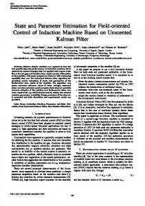
6.1 Simulations results The results of simulations show that the Luenberger observer gives an error tends to zero and the flux observed follows very well the real flux of the machine and has a better robustness as regards parametric variations (variations of rotor resistance). The results of simulations of robust control are present in (Fig. 9) and we note clearly that decoupling is maintained and the speed follows the reference well and is not affected by the application of a resistive torque.

7. Conclusion In this paper, we have studied the robustness of H  control applied to an induction motor and by using the Luenberger observer for the observation of rotor flux. The obtained results showed the robustness of the variables flux and speed against external disturbances and uncertainties of modelling. This method enabled us to ensure a good robustness/stability compromise as well as satisfactory performances. The use of the Luenberger observer enables us to avoid the use of the direct methods of measurements weakening the mechanical engineering of the system.

70


(a) (b) Fig. 8. Luenberger observer (a) with no variation of Rr and (b) with increase of Rr 100%

Fig. 9. Robust control with Luenberger observer

8. References Benchaib, A. & Edwards, C. (2000). Nonlinear sliding mode control of an induction motor. International Journal of Adaptive Control and Signal Processing, Vol.14, No.2-3., (Mar 2000) page numbers (201-221)


71

Chan, C. C., Leung, W. S. & Ng, C.W. (1990). Adaptive decoupling control of induction motor drives. IEEE Transactions on Industry Electronics, Vol.37, No.01, (Feb. 1990) page numbers( 41–47) De Luca, A. & Ulivi, G. (1989). Design of an exact nonlinear controller for induction motors. IEEE Transactions on Automatic Control, Vol. 34, No.12, (Dec 1989) page numbers (1304 – 1307) Marina, R. & Valigi, P. (1991). Nonlinear control of induction motors: a simulation study. European Control Conference, pp. 1057-1062, Grenoble, 2-5 July, France Nicklasson, P.J. Ortega, R. & Espinosa-Perez, G. (1997). Passivity based control of a class of Blondel-Park transformable electric machines. IEEE Transactions on Automatic Control, Vol.42, No.5, (May 1997) page numbers (629-647) Gokdere, L.U. (1996). Passivity based methods for control of induction motors. Ph.D. Thesis, University of Pittsburgh, 1996 Kanellakopoulos, I. Krein, P.T. & Disilvestro, F. (1992). Nonlinear flux observer based control of induction motors, American Control Conference, pp.1700–1704, Chicago, (June 1992). USA Abdel Fattah, H. A. & Loparo, K. A. (2003). Passivity based torque and flux tracking for induction motors with magnetic saturation. Auotmatica, Vol.39, No.12, (December 2003), page numbers (2123-2130) Peresada, S. Tonielli, A. & Morici, R. (1999).High-performance indirect field-oriented output-feedback control of induction motors, Automatica , Vol.35, No.6, (June 1999) page numbers (1033-1048) Barambones, O. Garrido, A.J. & Maseda, F.J. (2003). A sensorless robust vector control of induction motor drives. IEEE International Conference on Emerging Technologies and Factory Automation, Lisbon, (September 2003). Portugal Marina, R Peresada, S & Tomei, P. (1998).Adaptive output feedback control of current-fed induction motors with uncertain rotor resistance, Automatica, Vol. 34, No. 5, (Oct 1998) page numbers (617-624), ISSN 0005-1098 McFarlane, D. Glover, K. & Noton, M. (1988). Robust stabilization of a flexible space platform: an H∞ coprime factor approach, International Conference on Control, pp (677-682), ISBN 0-85296-360-2, Oxford, UK, April 1988. McFarlane, D. & Glover, K. (1988). An H design procedure using robust stabilization of normalized coprime factors, IEEE Conference on Decision and Control, pp (1343-1348), INSPEC 3371748, Austin, TX, USA, December 1988. McFarlane, D & Glover, K. (1989). Robust controller design using normalised coprime factor plant descriptions, lecture Notes in Control and information Sciences, Springer Verlag, (138), Berlin, Germany Glover, K. & McFarlane, D. (1988). Robust stabilization of normalized coprime factors: An explicit H∞ solution, IEEE International American Control Conference, pp(842 – 847), Atlanta, Ga, USA, June 1988. Glover, K. & McFarlane, D. (1989). Robust stabilization of normalized coprime factor plant descriptions with H bounded uncertainly, IEEE Transactions on Automatic Control, Vol. 34, No.08, (Aug.1989) page numbers (821-830) McFarlane, D. & Glover, K. (1992). A loop shaping design procedure using H∞ synthesis, IEEE Transactions on Automatic Control, Vol. 37, No.06, (June 1992) page numbers (759-769)

72


Blaschke, F. (1972). The principle of field orientation as applied to the new transvektor closed-loop control system for rotating-field machines, Siemens Review, Vol.34, pp ( 217–220), Mai 1972. Boukhnifer, M. (2007). Commande robuste d’une machine asynchrone alimentée par un à onduleur multi-niveaux, Revue Internationale en Génie électrique, Vol 10, No.06, (November –December 2007) page numbers (717-749). Orlawska-Kowalska, M. (1989). Application of extended luenberger observer for flux and rotor time constant estimation in induction motor drive. IEE Control Theory and Applications, Vol.136, No.6, (Nov 1989) page numbers (324–330), ISSN: 0143-7054