6th World Congresses of Structural and Multidisciplinary Optimization Rio de Janeiro, 30 May - 03 June 2005, Brazil
Stochastic Optimization Applied to R-C Building Grillages Moacir Kripka Department of Civil Engineering, University of Passo Fundo, Passo Fundo, RS, 99001-970, Brazil E-mail:
[email protected] Abstract This work presents a formulation developed to minimize the volume of concrete in reinforced concrete building grillages. An association of the displacement method with optimization techniques seeks to obtain the cross-sectional dimensions which lead to the smallest volume of concrete, attending to the ultimate loads (failure) and service loads (deflections). The constraints imposed in the formulation of the problem related to the limitation of the displacements include the effects of instantaneous and long-term deflections, considering an equivalent inertia with the contribution of concrete between cracking (Branson). The determination of the minimum height to each cross-section due to the flexural strength can be performed by fixing neutral axis position or by the maintenance of the section as underreinforced. Due to the relative complexity of the formulation as well as to the existence of local minimas, even for a small number of variables, a stochastic method was chosen, being implemented the Simulated Annealing. In order to verify the efficiency of the proposed procedure, some of the analyzed structures are presented, as well as the results obtained from the implementation of the proposed formulation. Keywords: simulated annealing, grillages, reinforced concrete, weight optimization. 1. Introduction The analysis and the dimensioning of structures, in a general way, constitute in procedures of high complexity. When involving a great number of variables, they need to be developed in an iterative way. Due to this characteristic, the values initially adopted to the variables depend on the determinative form of the sensitivity as well as of the previous experience of the designer. Still thus, the number of demanded analysis would be raised in case that it was desired to get the optimum values, among the universe of all possible and occasionally more economical alternatives. Describing, however, the physical behavior of the structure through mathematical functions, extreme values of such functions can be searched with the aim of optimization techniques. In a general way, a minimization problem can be expressed as: minimize f ( x i ) i = 1, n (1) subject to g j ( x i ) ≤ 0 j = 1, m (2) k = 1, l (3) hk(xi)=0 xil ≤ xi ≤ xiu (4) T where F designates the objective function and X = ( x1 , x2 , ... xn ) consists in the vector of the design variables. The other functions are called constraints of the problem (respectively inequality constraints g, equality constraints h and side constraints, with lower limit l and upper limit u). The functions involved in the problem may contain the design variables in an explicit form or not, and can be analytically or numerically developed. Objective function as well as restriction functions may be linear or non-linear. The great development of the structural optimization occurred in the beginning of the 60’s, when programming techniques were used aiming at a minimization of structures weight. From then on, a big diversity of general techniques was developed and adapted to structural optimization. The application of these approaches to the practical resolution of problems, however, has not been verified in the same proportion. Cohn et al. [1], based on more than 500 examples taken from articles and books, emphasize in their work the big worry with mathematical aspects of optimization, although the number of examples presented is very small, being these normally of purely academic interest. The main reason to the little application of optimization techniques to the practical problems of structural engineering consists of the complexity of the model generated, described by non-linear functions and generating a non-convex space of solutions (several points of optimum), problems for which the resolution by traditional techniques of mathematical programming has shown little efficiency. For the resolution of these kinds of problem, the heuristic methods have been performing an important role, since they involve only function values in the analysis, being not necessary the existence of unimodality or even continuity of their derivatives. Otherwise, they present as disadvantage the necessity of a big number of function evaluations. This disadvantage, however, is questioned by some researchers like Powell [2] who argues that, instead of performing additional number of calculations for the numerical determination of the gradient when mathematical programming is being used, these number of calculations can be performed to exploit more intensely the space of solutions. Among the main heuristic methods, the growing application of Simulated Annealing can be verified. It consists in an approach to global optimization developed in analogy upon the mechanic procedure of annealing of the metals. Still little employed in the structural optimization, Simulated Annealing is of easy computational implementation, dealing with few control parameters regarding the Genetic Algorithms. The present work shows an application of Simulated Annealing to the optimization of crosssections of structural elements of buildings in reinforced concrete, analyzed by the grillage model. Even if due to limitations of economic and aesthetic order only a reduced number of distinct cross-sections for the beams can be considered, the possible number of combinations is enough elevated. Because the model has a high degree of indeterminacy, the stresses are redistributed by altering the relative stiffness of the elements when a cross-section of a single beam is changed.
Several works related to the optimization of reinforced concrete beams can be found on technical literature. The results obtained from the present work, however, indicate that the sum of local optimums resultant from the analysis of isolated beams does not coincide with the minimum obtained when the procedure is applied to all the elements simultaneously. Former studies developed by the author [3] concluded that similar results can be achieved considering as the design variables the costs of reinforcement, concrete and formworks. By taking the minimum volume (or weight) of concrete as objective, nevertheless, the problem become independent of regional variations. 2. Simulated Annealing Method The optimization approaches normally employed are based in descending strategies. In these, from an initial solution, a new solution is generated and the value from the function obtained for this solution is compared to the initial one. If a reduction in the function value is verified, this new value passes to be adopted as the current solution and the procedure is repeated until any better value to the function can be obtained. The final result obtained, depending on the characteristics of the functions involved, can be the best solution in the neighborhoods from the initial solution, but not necessarily the best in the search space. An usual strategy to improve the solution obtained consists of the analysis of the problem from several initial solutions. Simulated Annealing utilizes a different strategy, trying to avoid convergence to a local minimum accepting also, according to a specific criterion, solutions that increase the value of the function. The method is recognized as a procedure for obtaining good solutions for optimization problems of difficult resolution, developed in analogy upon the process of annealing of a solid, when a state of minimum energy is being searched. The denomination annealing is given to the process of heating of a solid to its point of fusion, followed by a slow cooling. In this process, slow cooling is essential to maintain a thermal equilibrium in which the atoms are able to reorganize themselves in a structure with minimum energy. If the solid is cooled abruptly, its atoms will form an irregular and weak structure, with high energy in consequence of the internal effort spent. In computational terms, the annealing can be seen as a stochastic procedure of determination of the organization of the atoms with minimum energy. To high temperatures the atoms move themselves freely being able to, with big probability, achieve positions that will increase the energy of the system. When the temperature is reduced, the atoms can move themselves gradually to form a regular structure, and the energy increase probability is reduced. According to Metrópolis et al. [4], the probability of changing in the energy of the system is given by
⎛ − ∆E.K ⎞ p(∆E) = exp⎜ (5) ⎟ ⎝ T ⎠ were T is body temperature and K the Boltzmann constant. The simulation of annealing as an optimization technique was originally proposed by Kirkpatrick et al. [5], in which the objective function corresponds to the energy of the solid. Similarly to the annealing in thermodynamics, the process initiates with a high value of T, for which a new solution is generated. This new solution will be automatically accepted if it generates a decrease in the value of the function. Being the new value of the function greater than the previous one, the acceptation will be given according to a probabilistic criterion, being the acceptation function ⎛ − ∆f ⎞ p = exp⎜ (6) ⎟ ⎝ T ⎠ and the new solution accepted if p is bigger than a number between zero and one, generated randomly. While T is high, the majority of the solutions is accepted, being T reduced gradually to each trial series, in the neighborhood of the current solution. 3. Formulation to the Minimization of the volume of Concrete The goal defined by the developed formulation consists in the minimization of the volume of concrete of linear elements on a building floor, and can be written as f = Σ (bwi hi li) i=1,n (7) being n the total number of elements and bwi , hi and li , respectively, the width, the height and the length of i-esim element. Since the number of different cross-sections on the same floor is restrict, the number of design variables is very low when related to the number of elements. In this way, while the number of terms of the objective function is equal to the number of elements of the floor, each of the constraints is applied only m times, being m the number of distinct cross-sections. The first constraints imposed to the problem are related to service limit state, being considered only the limitations on maximum deflections. The maximum deflection dmax in each element is determined with the consideration of long term loads, to which are added the displacements obtained by the consideration of the cracking of concrete. This maximum deflection is limited by dadm, or admissible deflection. Regarding the maximum bending moments, constraints were considered related to the minimum height to each group of elements. With this purpose hj is defined as the height assigned to the group and hmin the minimum height needed for the maintenance of the cross-section as underreinforced. In function of the above considerations, the problem was formulated as: min f = Σ (bwi hi li) i = 1,n (7) s.t. g1 = δmax j - δadm ≤ 0 (8) g2 = hmin - h j ≤ 0 j = 1,m (9) The consideration of the constraints in the computational implementation was made by using a dynamic penalty technique, known as annealing penalty [6]. Similar to the optimization technique, a penalty factor has an initial value relatively low, which is gradually increased due to the temperature reduction. In this way, the penalized function F (x) can be written as: F (x) = f(x)+P(x) (10) being
⎛ 1 ⎞ P( x ) = ∑ ⎜ (11) ⎟ g(x ) 2 ⎝ 2T ⎠ where P (X) is the function which represents the assembly of the penalized constraints. In this way, even if the problem starts from unfeasibles solutions, small violations of constraints are initially allowed.
4
4.00 m
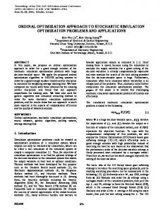
4. Examples The described formulation was implemented on a software developed for the analysis of grillages by the Displacement Method, in which was inserted a routine of optimization developed in the form proposed by Cornana et al. [7]. In this way, both the data input and the form of presentation of the results are familiar to the engineer used to structural analysis software. A separate file with the description of the evolution of the optimization process is generated. Material properties (longitudinal and transversal modules of elasticity) are evaluated automatically from the input, by the user, of the value of the strenght of the concrete. The initial height of the cross-section can be supplied by the user or estimated automatically. Since that value constitutes the initial solution to the optimization problem, it little influences the result. From these initial heights, flexural and torsional rigidity (these last ones reduced to consider cracking of the concrete) are calculated. Finally, dead and live loads should be supplied separately, being the own weight computed automatically. Although the dimensioning of the elements was made according to Brazilian Code [8], it can be supposed than the conclusions made in this work are still valid by the application of other design codes. In the sequence of this work, some of the examples analyzed from the implementation of the proposed formulation are presented. The objective of this analysis was to study the behavior of the selected structures and the verification of the effectiveness of the employed technique. In all of the examples the height of the elements was limited to do not drive to overreinforced sections, being the flexional rigidity determined from the expression proposed by Branson [9]. The first analyzed structure, illustrated in Figure 1, consists of a grillage composed by two simply-supported beams, both with a total length of eight meters. The total load, considered only as dead load, is of 24 kN/m uniformly distributed, being the own weight computed automatically. The width of all the elements was set to 20 centimeters, being the heights the design variables. Regarding to the material properties, concrete C-20 and steel CA-50A were considered.
2
3
4.00 m
1
4.00 m
4.00 m
Figure 1. Example 1 Starting from the same initial height for all elements, taken as 0,80 meters, and by imposing to all of them the same final dimensions, it was obtained a reduction of about 24,3 percent in the volume of concrete Vc, according to Table 1. In this same table, it can be observed the bending moments and maximum displacements obtained (Mmax and dmax, respectively) being the bending moments in the central nodes determinant for the limitation of the height of the beams (the displacements listed already take into account longterm effects). Table 1. Example 1: initial and optimum heights
Initial Optimum
h (m) 0.8000 0.6055
Vc (m3) 2.560 1.938
Mmax (kN.m) 224.00 216.22
δmax (cm) 1.003 2.468
The same structure was analyzed considering two design variables, limiting elements 1 and 2 to the same height h1 and elements 3 and 4 to height h2. By the analysis of this situation two points of global optimum were obtained, due to the symmetry. It can be verified that the situation previously illustrated, for which all the elements assumed the same final cross-sectional dimensions, corresponds to a point which satisfies the constraints of the problem, however consisting in a local minimum. The situation described can be visualized with the aid of Figure 2, where the straight lines represent the objective function (total volume of concrete) and the curves represent the active constraints gm and gd (minimum heights for moments and deflections for each beam). In this way, the values from the function that attend simultaneously all constraints are situated above the curves of highest value for each pair of coordinates (h1,h2). For all of them, bending moments limit the height of the elements (active constraints).
0.9
5 2,
0 2,
C
A
0.8 0.7
B
0.6
h2 (m)
5 1, 0.5 0.4
C 0.3
0.4
0.5
0.6
0.7
0.8
0.3
0.9
h1 (m) g δ= 0
g m= 0
f
Figure 2. Example 1: two design variables Still based on Figure 2, despite the fact that the objective function is linear, the constraints of the problem are non linear, generating a non convex region and, therefore, being susceptible to the existence of local minimums. The coordinates of points assigned in the figures by the letters A (initial volume), B (local minimum) and C (global minimum), as well as the corresponding absolute and relative, are listed in Table 2. It can also be observed that, even if the structure presents symmetry, the situation that drives to the smallest volume of concrete does not correspond to the same height for the cross-sections of the elements. Table 2. Example 1: initial and optimum heights
Initial Local opt Global opt
h1 (m) 0.8000 0.6055 0.8746 0.2651
h2 (m) 0.8000 0.6055 0.2651 0.8746
Vc (m3) 2.560 1.938 1.824 1.824
Vc / Vc ini 1.000 0.757 0.712 0.712
By solving an elementary optimization problem, the conclusion made above can be generalized. Considering, e.g., the same structure in Figure 1, where now the gol is to minimize its stiffness (or the sum of moments of inertia) to the same total weight (or sum of elements height H constant). I we take the sections h1 and h2 as the design variables the new problem can be formulated as: min f = Σ (Ii) i = 1,2 (12) (13) s.t. Σ hi = H The analytical solution to this problem, simplified to rectangular cross section of width b leads to
(
) 12 [
f = b h13 + h 32 = b h13 + (H − h 2 )3 12
∂f = 0 ∂h1
→ h1 = h 2 = H 2
]
(14) (15)
Since b and h are nonnegative, is can be verified than the same height to the elements represents the minimum stiffness to the structure. Therefore, a small reduction in h1 with the same amount of material added to h2 will stiff the structure as a whole. The other structure analyzed presents two axes of symmetry, and it is composed by ten beams, or forty elements (see Figure 3). In this structure, the actions are taken from slabs which were submitted to a uniformly distributed load of 4.5 kN/m2 (being 1.5 kN/m2 due to live loads), and from a uniformly distributed load of 3.6 kN/m applied along the external beams (V1, V5, V6 and V10). The weight of the beams was computed automatically. The width of all beams was fixed (0.20 meters). Again, concrete C-20 and CA50A steel were considered.
V1
4 x 3.00 m = 12.00 m
V2
V3
V 10
V9
V8
V7
V6
V4
V5
4 x 3.00 m = 12.00 m
Figure 3. Example 2: typical floor Initially all beams were limited to the same height, therefore constituting a problem with an only variable and two constraints. Starting from an initial height of 0.80 meters, an optimum height of 0.6485 meters was obtained, corresponding to a reduction in the volume of concrete of about 18.9 percent (Table 3). As it can be verified from the table, the height was limited in function of the vertical displacement on the central node. Table 3. Example 2: single design variable h (m) 0.8000 0.6485
Initial Optimum
Vc (m3) 19.200 15.565
Mmax (kN.m) 227.06 211.16
δmax (cm) 2.180 4.000
Following the supposition that the new determined height consists only in a local minimum, another analysis was performed, in order to verify the effective reduction on concrete consumption starting from this situation (assigned as case A). It can be stressed that, since the adopted method accepts movements which increase the value of the function, it is weakly dependent of the starting point. New situations were analyzed as follows: -External beams with height h1 and internal beams with height h2. Assigned as case B, with two design variables; -External beams with height h1, internal beams (horizontal, V2 to V4) with height h2 and internal beams (vertical, V7 to V9) with height h3 (case C, three design variables); -Each beam being able to assume a different height (case D, ten design variables); -Each element being able to assume a different height (case E, forty design variables). Table 4 presents the results obtained for the cases B and C, comparing the reduction on the volume of concrete obtained relatively to case A and to fixed height of 0.80 meters (assigned as case 0). Table 4. Example 2: up to tree design variables case 0 A B C
h1 (m) 0.8000 0.6485 0.4168 0.5137
h2 (m) 0.8000 0.6485 0.6834 0.1659
h3 (m) 0.8000 0.6485 0.6834 0.7858
Vc (m3) 19.200 15.565 13.842 11.784
Vc / Vc(0) Vc / Vc(A) 1.000 1.234 0.811 1.000 0.721 0.889 0.614 0.757
From the previous results presented, it can be concluded that since the height of the internal beams can not be reduced more than in case A due to the deflection limitation, it can be advantageous to free the external beams to assume another height, since their lengths are smaller than the internal ones. In addition, it can be verified that despite the symmetry of the structure, a more economic situation is obtained by permitting the perpendicular internal beams to assume different heights, increasing the total stiffness without reducing the concrete consumption or, as the presented case, by the maintenance of the original stiffness with reduction in the consumption (about 24.3 percent regarding case A, as indicated). It must be remembered that the optimum for case C is obtained equally by the inversion of h2 and h3. Generally, it was verified a significant increase on the number of local minimum points due to the increase in the number of distinct cross-sections allowed (e.g., the optimum obtained to cases A and B are local minimum of the case C, and so on). Because of that, as well as the practice limitation of different cross-sections to a reduced amount, the results of the analyses performed to bigger number of variables are presented separately.
Since Simulated Annealing method is based on probabilities, and since its results are function of pseudo-random numbers, the success of this method is directly related to both the complexity of the problem and to the adjustment of the parameters. In this way, in order to verify the constancy of the results, the analysis of the problem containing 10 design variables was performed 100 times. The results of this problem, assigned as case D, were obtained by allowing all the beams to assume different heights, and can be resumed as follows: Initial Volume: 19.200 m3 Worst result: 11.124 m3 Average: 9.001 m3 Best result: 8.819 m3 Frequency of best result: 70 % Number of function evaluations (average): 24,631 Reduction in volume (in relation to case 0): 54.1 % Reduction in volume (in relation to case A): 43.3 % The final heights corresponding to the smallest volume obtained are presented in Table 5, remembering that due to double symmetry of the structure another combination drove to the same final volume. It can be observed that the heights are alternated in a way that there are no beams with the same height in each crossing (node). It can also be verified the great height assumed by one of central beams (V8), with the consequent relief of the beams immediately adjacent (V7 and V9). Regarding the number of occurrences of the best result, this number can be highly increased by increasing also the initial temperature. However, this will probably lead to a great number of function evaluations until the convergence is achieved. Analogous procedure was adopted to the analysis of the same structure considering 40 design variables (each element being allowed to assume a distinct height). Summary of the results: Initial Volume: 19.200 m3 Worst result: 11.123 m3 Average: 8.795 m3 Best result: 8.403 m3 Number of function evaluations (average): 106,921 Reduction in volume (in relation to case 0): 56.2 % Reduction in volume (in relation to case A): 46.0 % Reduction in volume (in relation to case D): 4.7 % Table 5. Example 2: optimum height (10 design variables) beam V1 V2 V3 V4 V5 V6 V7 V8 V9 V10
h (m) 0.299 0.336 0.303 0.336 0.299 0.359 0.128 1.129 0.128 0.359
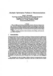
Regarding the number of function evaluations needed to the solution of the problem with Simulated Annealing, it can be clearly observed that this number is very high when compared to those obtained by mathematical programming. Therefore, this approach is specially indicated to problems in which the usual techniques are not efficient. Nevertheless, it was observed that Simulated Annealing, when applied to the examples of the present work, leads rapidly to the neighborhoods of the optimum solution. Figure 4 presents the results obtained to case D, being possible to observe that after 4400 function evaluations the error is lower than 1 percent. In this way, a definition of a less rigorous stop criterion can drive to a significant reduction in the number of calculations.
2.2 2
Vc ini / Vc *
1.8 1.6 1.4 1.2 1 0
5000
10000 15000 function evaluations
20000
25000
Figure 4 - Example 2: convergence to 10 design variables 5. Concluding Remarks This work presented a formulation to the determination of minimum volume of concrete in structures analyzed by the grid model. Since the determination of the cross-section dimensions of the elements is performed mainly based on the former experience of the designer, the program developed from the proposed formulation can constitute a valuable tool in the phase of dimensioning, allowing the designer to identify the more stressed elements as well as those that eventually could be deleted from the structure. Considering the iterative character of the structural dimensioning, and also the high degree of indeterminacy of building grillages, the application of optimization techniques to the problem was found to be very adequate. In this sense, it was also verified the applicability of Simulated Annealing to this kind of problem, specially due to the existence of local minimums even for a small number of variables. In the present work just symmetrical structures were analyzed, for which it was supposed that the final configuration should drive to identical cross-sections for equally loaded elements. The obtained results, however, suggest that the relative alteration in the dimensions of the elements can lead to a reduction in the volume of concrete without reduction in the global stiffness. 6. References 1. Cohn, M. Z.; Fellow; Dinovitzer, A. S. Application of structural optimization. Journal of Structural Engineering, ASCE, 1994, v.120, n.2, p.617-50, Feb. 2. Powell, M.J.D. Direct Search Algorithms for Optimization Calculations. Numerical Analysis Report, DAMTP 1998/NA04, Department of Applied Mathematics and Theoretical Physics, Silver Street, Cambridge, England CB3 9EW, march 1998. 3. KRIPKA, Moacir. Minimum Cost of Reinforced Concrete Building Grillages by Simulated Annealing. In: WCSMO-5 - THE FIFTH WORLD CONGRESS OF STRUCTURAL AND MULTIDISCIPLINARY OPTIMIZATION, 2003, Lido di Jesolo, Veneza. Short papers of the fifth world congress on Structural and Multidisciplinary Optimization. Milão: Italian Polytechnic Press, 2003. p. 407-408. 4. Metropolis, N.; Rosenbluth, A.; Rosenbluth, M.; Teller, A.; Teller, E. Equation of State Calculations by Fast Computing Machines. J. Chem. Phys. , 1953, 21, 1087-1090. 5. Kirkpatrick, S.; Gelatt, C. D.; Vecchi, M. P. Optimization by Simulated Annealing. Science, 1983, 220, 4598, 671-680. 6. Michalewicz, Z. and Schoennauer, M. Evolutionary Algorithms for Constrained Parameter Optimization Problems. Evolutionary Computation, MIT Press, 1996, 4(1): 1-32. 7. Corana, A.; Marchesi, M.; Martini, M.; Ridella, S. Minimizing Multimodal Functions of Continuous Variables with Simulated Annealing Algorithm. ACM Transactions on Mathematical Software, 1987, 13, 262-280. 8. Associação Brasileira de Normas Técnicas. 'NBR 6118 - Projeto e execução de obras de concreto armado'. Rio de Janeiro, ABNT, 1978. 9. Branson, D. E. Instantaneous and Time-Dependent Deflection of Simple and Continuous RC Beams, Alabama Highway Research Report, n. 7, Bureau of Public Roads, 1963.