Mark Gerrits, Bert De Decker, Cosmin Ancuti, Tom Haber, Codruta Ancuti, Tom Mertens, ..... [3] Iddo Drori, Daniel Cohen-Or, and Hezy Yeshurun, âFragment-.
STROKE-BASED CREATION OF DEPTH MAPS Mark Gerrits, Bert De Decker, Cosmin Ancuti, Tom Haber, Codruta Ancuti, Tom Mertens, Philippe Bekaert Hasselt University - tUL -IBBT, Expertise Center for Digital Media, Wetenschapspark 2, Diepenbeek, 3590, Belgium ABSTRACT Depth information opens up a lot of possibilities for meaningful editing of photographs. So far, it has only been possible to acquire depth information by either using additional hardware, restrictive scene assumptions or extensive manual input. We developed a novel user-assisted technique for creating adequate depth maps with an intuitive stroke-based user interface. Starting from absolute depth constraints as well as surface normal constraints, we optimize for a feasible depth map over the image. We introduce a suitable smoothness constraint that respects image edges and accounts for slanted surfaces. We illustrate the usefulness of our technique by several applications such as depth of field reduction and advanced compositing. 1. INTRODUCTION Altering the appearance and content of images is a challenging task. Over the past years, we have seen tremendous progress on this front: it is possible to add, edit and remove objects [1, 2, 3, 4, 5] in photographs; and to transform [6], to enhance [7, 8] and even to animate [9] them. Even though meaningful editing is already possible, such tools are often limited by the fact that a photograph is only a flat, 2-dimensional depiction of the world. We present a technique for enriching existing photographs with depth information, which will permit more advanced editing operations, like decreasing depth-of-field, occlusion-aware compositing, and so on. Our work builds on previous techniques for adding geometric information to images [10] and single-view modeling [11, 12]. We also are inspired by techniques using scribble or stroke based input [13, 14, 15]. Such methods require only sparse user input, and propagate information while respecting object boundaries. The main contribution in this paper, is an optimization technique for painting depth maps from stroke-based input, as was done for colorization [14] and for tonal adjustment [15]. However, to the best of our knowledge, we are the first that employ strokes to estimate the depth. Since humans are not very efficient at estimating absolute depth [16], we also introduce “normal” strokes, which enable the user to place surface orientation constraints. This allows for easy creation of
slanted regions. Our technique simultaneously respects these two types of constraints within the same optimization framework. Our tool is not intended to produce precise depth information at an absolute scale, but we strive to produce plausible, smooth depth maps that contain consistent object boundaries. These maps can be used to achieve alterations that would be hard to realize without depth information. We demonstrate the following effects in this paper: depth-of-field adjustment, occlusion-aware compositing and adding fog. 1.1. Related Work A considerable amount of work has focused on acquiring accurate depth information from real-world scenes using specialized hardware setups. Stereo techniques use two [17] or more [18] cameras, and estimate per-pixel disparities between the different views. Structured light [19] uses one or more cameras to examine a scene lit by a projector that emits coded illumination. These techniques aim at faithful reconstruction of geometry, and always require special hardware, often in laboratory conditions. This limits their applicability, as the setup is not always portable, and may not work when external illumination is present. Since we merely want to edit the image, we do not necessarily need a very accurate reconstruction. Single-view modeling is closely related to our goal. Khan et al. [5] seek to reconstruct a coarse shape for editing material appearance. They map luminance values directly to depth, which does not always produce plausible results. Since the effect of the depth values is not directly visible in the final image, it is adequate for their purpose. A similar technique has been used in other image-based modeling tools [11] to realize local editing operations, but it is not reliable enough to be used as a general technique to estimate shape. Boulanger et al. [20] automated the selection of vanishing points. The resulting scene geometry is very coarse but suited for walkthroughs, especially in typical urban scenes, consisting of roads and buildings. Our tool is more general, and can be applied to non-urban scenes as well. Boiem et al. [21] model a scene as a ground plane and a collection of vertical billboards, similar to a pop-up picture. They learn appearance of canonical parts in photographs, like “ground” and
“sky”, and reconstruct a scene accordingly. Their technique is limited to simple outdoor scenes, and requires a database of hand-labeled examples. Oh et al. [11] create depth using a variety of specialized operations, such as “rgb to depth” [22], image processinginspired filters, a generic model for fitting human faces, and a chiseling brush. These tools model variety of scenes, but still require many hours of labor from the user. Zhang et al. [12] optimize for a desired depth map using point-wise depth, normal and silhouette constraints. Unfortunately, the user still has to perform many interactions before a detailed reconstruction is obtained. We seek to compute an optimal depth function, given a set of user-supplied constraints in the form of strokes, and a smoothness constraint. This strategy has been employed before to solve vision and graphics problems with user assistance. Boykov et al. [23] and Rother et al. [13] use graph cut optimization to segment foreground elements in images, based on an initial user-specified segmentation. Levin et al. [14] colorize grayscale images using a few colored scribbles. Okabe et al. [10] use a similar strategy to propagate normals across images for relighting. Lischinski et al. [15] propagate tonal adjustment across an image. Our work is different from previous stroke or scribble-based techniques, in that our objective function simultaneously incorporates absolute constraints on the unknown function (depth), and on its derivative (surface normals). 2. PAINTING WITH DEPTH We want to provide a way for users to assign depth values to pixels in such a way that they have to provide as little input as possible. A stroke-based user interface in which the users only have to draw a few broad strokes, provides a good means to this end. In our implementation, the user can specify absolute depth constraints and normal constraints in an intuitive manner. The normal constraints are converted to constraints on the gradient of the depth map. The depth maps should be of sufficient quality for a wide array of rendering applications. For this, it’s important that the depth values are interpolated across the image in such a way that depth discontinuities are preserved and the depth values are allowed to vary smoothly across slanted planes. We accomplish this by optimizing an energy function over the image that takes into account the user constraints and addresses these concerns with a suitable smoothness term.
Fig. 1. Example of user input. About a minute was spent specifying the constraints. 7 strokes were drawn. Absolute depth constraints appear as greyscale strokes. Normal constraints are illustrated by textured strokes and a shaded, blue 3D vector. Absolute depth brush strokes are visualized either with a greyscale intensity value corresponding to their depth value or textured with a checkerboard pattern which is scaled according to the depth value. The choice is left to the user, according to which he finds more intuitive. For the greyscale representation, darker intensities correspond to areas closer to the viewer while lighter intensities belong to areas which are farther away. For the checkerboard representation, a more zoomed in pattern with larger boxes indicates nearby regions, while a zoomed out texture lies naturally at a farther distance. The user specifies the required depth value with a simple slider. For the normal constraints, the user specifies the normal of a plane that is coplanar with the surface represented by the pixels covered by the brush stroke. The normal can be easily specified by dragging the end point its projection in the 2D image plane. The constraint is visualized by a shaded 3D vector and a checkerboard pattern which is warped according to the normal to coincide with the surface element. An example of a set of user-defined brush strokes can be seen in figure 1. 2.2. From normals to gradients
2.1. User controls The user is presented with an interface which allows him to easily scribble two kinds of strokes: those that define absolute depth constraints and those that define normal constraints. The constraints are applied to all pixels that are covered by the respective brush strokes.
The optimization, as described in the next section, works on depth values and not a direct scene geometry. Therefore it is useful to convert our normal constraints which directly describe the 3D scene to gradient constraints which directly describe the changes in depth values. Since the normals are given in 3D camera coordinates,
Input image
Depth without gradient constraints
Depth with gradient constraints
Fig. 2. Depth estimation. Without gradient constraints, slanted surfaces are disrupted by texture information or suffer from sub-optimal depth distribution. while the gradients we are looking for are in image coordinates, we need to perform a mapping from the 3D camera coordinates to the 2D image coordinates. For a normal n with camera coordinates (n x , ny , nz ), 2D pixel coordinates (ni , n j ) and depth n d ∈ [0, 1], (−nd , n j , ni ) and (ni , −nd , n j ) are the perpendicular vectors that lie in the X and Y plane respectively. Therefore, the gradient corresponding to this normal is grad(n) = (−n i /nd , −n j /nd ). The normal can be mapped from camera coordinates to image coordinates with the formula (n i , n j , nd ) = ( fi , f j , fd )(nx , ny , nz ), where f i , f j and f d are parameters that depend on internal camera parameters and the positions of the nearest and farthest depth plane. n This means that grad(n) = (−α i nnxz , −α j nyz ), with αi = ffdi and fj fd .
αj = If the coordinates of two pixels a = (a i , a j , ad ), b = (bi , b j , bd ) are known in image coordinates along with the normal n = (n x , ny , nz ) in camera coordinates of a plane through both points, it is possible to calculate α i and α j in a few simple steps: ni f i nx bi − ai = = nd f d nz bd − ad nx bi − ai = nz bd − ad nz bi − ai αi = nx bd − ad
αi
and similarly for j:
αj =
nz b j − a j ny bd − ad
2.3. Optimization Our goal is to compute a function f which assigns a depth value to each pixel of the image. This function is required
to follow the user-specified constraints as closely as possible. As depths often vary smoothly in the real world, it is also important to impose a certain degree of smoothness to the depth function in order to construct a good depth map. However, depth discontinuities should still be allowed at object boundaries. These boundaries are often characterized by sudden shifts in pixel colours. Thus, the function we’re trying to determine can be found by minimizing the following energy function: E( f (x)) = ∑(D(x) + λ V(x)) x
D is the data term, V is the smoothness term and λ decides the relative importance of both terms. The data term is responsible for keeping f close to the user-specified constraints. The user can specify two sorts of constraints, each codified in their own data term: D(x) = A(x) + ϕ G(x) A is the absolute data term, G is the normal data term and ϕ regulates the relative weight of both terms. The absolute data term encourages the function to stay close to the absolute value constraints provided by the user: A(x) = wa (x)( f (x) − k(x))2 The weight wa indicates for which pixels constraints are provided by the function k and how much influence they exert. Similarly, the normal data term constrains the gradient of f to the user-specified gradients: G(x) = wg (x)(
∂ f (x) ∂ f (x) − gu(x))2 + wg (x)( − gv (x))2 ∂u ∂v
For many graphics optimization problems, the smoothness term will try to keep the gradient of the function as small
Input image
Real depth of field photo
Focus on second apple
Focus on third apple
Depth map
Focus on forth apple
Fig. 3. Shallow depth of field. A scene is rendered with shallow depth of field, focused at different depths. The bottom row shows our rendered results. A real shallow depth of field photo is also included for comparison. as possible wherever the image gradient is low. Where the image gradient is larger, the gradient of the function is allowed to increase. A smoothness term such as this favours functions that change their value as little as possible, except at colour discontinuities, which is what is often required. For the concrete case of depth painting, this would produce depth maps with planar regions orthogonal to the viewing direction. The real world, however, is not a series of layers aimed in our direction. Therefore we choose to use the weighted laplacian instead of the first derivative. A smoothing term based on the laplacian will favour areas with constant slope. Not only does this match the real world more closely (the ground, walls, ...) and have more tolerance towards areas with arbitrary curvature, it also better supports the normal data term. Using finite differencing we get: V (x) = ( f (x) −
∑y∈N4 (x) h(x, y) f (y) 2 ) ∑y∈N4 (x) h(x, y)
h(x, y) = e
(L −L )2 − x 2y 2σ
After applying finite differencing to the derivatives of f , E( f (x)) gives a quadratic expression in f , which can be minimized by solving the linear system:
result. This choice is not inherent to our algorithm, any suitable optimization technique could be used. 3. RESULTS AND DISCUSSION 3.1. Depth estimation As was previously mentioned, the main goal of our userassisted technique is to estimate adequate depth maps with an intuitive stroke-based user interface. In our experiments we used photographs taken with a commercial digital camera (Canon EOS 40D 10.1MP). Examples of our depth estimation results can be seen in figures 2 and 3 (top-left) (please refer as well to the supplementary material). Our unoptimized code (Matlab implementation) takes about 80 seconds to generate the depth map for a 320x240 image. All the generated results have been generated by choosing the default parameters of λ = 0.05, σ = 0.02 and ϕ = 0.2. Moreover, in our experiments we used 6 pyramid levels in the hierarchical scheme and ran the optimizer for 1000 iterations at each level. Figure 2 shows the importance of our normal constraints. They allow for easy generation of smooth depth maps and diminish the disruptive influence textures can have on the depth values of smooth 3D surfaces.
Af = b which is further detailed in the appendix. We hierarchically solve the system, starting at a course level and propagating the previous result to the finer levels. At each level we use the symmetric LQ method to obtain the
3.2. Applications As will be shown in the following, our tool has shown utility for several applications:
Input image
Foggy
Very foggy
Fake fog
Fig. 4. Synthesizing fog. Fog is added to a scene in different degrees. In the last image, fog is faked by just adding a gradient to the image in Photoshop. Our results are far more convincing. Shallow Depth of Field. The most common and simple way to use shallow depth of field is to simply bring the foreground element into focus and blur the background. Figure 3 shows the results of shallow depth of field rendering with our depth maps. By using the input image (top-left) we are able to estimate the depth map, which in turn was used to create the shallow depth of field rendering.The bottom row of the same figure shows the same scene with the focus placed at different depths. In the middle of the top row is shows a real photo of the same scene with shallow depth of field for comparison. Synthesizing Fog. Adding fog/haze to real photos is employed in several stylization tasks. In figure 4 (the two middle images) we use the depth information to add fog to a field of cows. For comparison we also made a fog image by adding a white gradient to the image in Adobe Photoshop, a technique often sued to simulate fog. As can be seen when comparing last tow images, our results looks more natural. Image Compositing. When using commercial software tools, combining multiple images into a single scene requires solid technique. In figure 5, we composite a chair into a new scene. As can be seen in the result image, the chair looks quite naturally at place in the scene. When creating the depth map for the chair, we gave the floor and wall a disproportionally large depth, allowing us to add the chair into the new scene without any need for segmentation. 4. CONCLUSION We have described a novel tool which allows users to easily create depth information for an existing photograph. Our technique optimizes for a smooth depth map in an edge-aware fashion, while taking into account stroke-based constraints imposed by the user. Besides absolute depth values, strokes may be used to specify local surface orientation (normals) in order to more easily define slanted regions. Our tool enables the user to create plausible depth maps with only a sparse set of strokes. We illustrated the usefulness of our technique by applying three depth-based effects on photographs: decreas-
ing depth-of-field, adding fog and occlusion-aware composition. Our tool would greatly benefit from interactive feedback. This could be made possible with an optimized implementation, or a more advanced solver [24]. Our gradient strokes tend to be useful for creating large planar geometry. We would also like to provide the user with a stroke that can assist in creating organic and curved shapes. 5. APPENDIX: ALGORITHM ⎧ λ h(i, �(i))h(�(i), j) ⎪ ⎪ ⎪ ⎪ ⎪ ⎪ ⎪ ⎪ λ h(i, �1 (i))h(�1 (i), j) ⎪ ⎪ ⎪ ⎪ +λ h(i, �2 (i))h(�2 (i), j) ⎪ ⎪ ⎪ ⎪ ⎪ ⎪ ⎪ ⎪ λ h(i, j) ∑k∈N4 (i) h(i, k) ⎪ ⎪ ⎪ ⎪ ⎪ −λ h(i, j) ∑k∈N4 ( j) h( j, k) ⎪ ⎪ ⎪ ⎪ −ϕ wg (i) ⎪ ⎪ ⎪ ⎪ ⎨ λ h(i, j) ∑k∈N4 (i) h(i, k) Ai j = ⎪ ⎪ λ h(i, j) ∑k∈N4( j) h( j, k) − ⎪ ⎪ ⎪ ⎪ ⎪ −ϕ wg ( j) ⎪ ⎪ ⎪ ⎪ ⎪ ⎪ ⎪ ⎪ wa (i) + 2ϕ wg (i) ⎪ ⎪ ⎪ ⎪ ϕ w + g (l(i)) + ϕ wg (u(i)) ⎪ ⎪ ⎪ ⎪ +λ (∑k∈N4 (i) h(i, k))2 ⎪ ⎪ ⎪ ⎪ +λ ∑k∈N4 (i) (h(i, k))2 ⎪ ⎪ ⎪ ⎪ ⎪ ⎪ ⎩ 0 and
j = �(�(i)), � = l ∨ r ∨ u ∨ d j = �1 (�2 (i)) �1 = l ∨ r, �2 = u ∨ d j = r(i) ∨ j = d(i)
j = l(i) ∨ j = u(i))
i= j
otherwise
wa (i)k(i) − ϕ wg (i)(gx (i) + gy (i)) j = l(i) bi = +ϕ wg ( j)gu ( j) j = u(i) +ϕ wg ( j)gv ( j) N4 (i) is the 4-pixel neighbourhood of pixel i. l(i), r(i), u(i) and d(i) are the pixels to the left, right, above and below pixel i respectively. 6. REFERENCES [1] William A. Barrett and Alan S. Cheney, “Object-based image editing,” in SIGGRAPH, ACM Trans. on Graphics, 2002, pp. 777–784.
relighting with normal map painting,” in Proceedings of Pacific Graphics 2006, October 2006, pp. 27–34. [11] Byong Mok Oh, Max Chen, Julie Dorsey, and Frédo Durand, “Image-based modeling and photo editing,” in SIGGRAPH, ACM Trans. on Graphics, 2001, pp. 433–442.
Input image
Chair
[12] Li Zhang, Guillaume Dugas-Phocion, Jean-Sebastien Samson, and Steven M. Seitz, “Single view modeling of free-form scenes,” in IEEE Conference on Computer Vision and Pattern Recognition (CVPR), 2001, pp. 990–997. [13] Carsten Rother, Vladimir Kolmogorov, and Andrew Blake, “”grabcut”: interactive foreground extraction using iterated graph cuts,” SIGGRAPH, ACM Trans. on Graphics, vol. 23, no. 3, pp. 309–314, 2004. [14] Anat Levin, Dani Lischinski, and Yair Weiss, “Colorization using optimization,” in SIGGRAPH, ACM Trans. on Graphics, 2004, pp. 689–694.
Composite image
Fig. 5. Image composite. A new element (a chair) is added to an existing scene. Both the original scene and the chair were assigned depth values with our technique. [2] Patrick P´erez, Michel Gangnet, and Andrew Blake, “Poisson image editing,” in SIGGRAPH, ACM Trans. on Graphics, 2003, pp. 313–318.
[15] Dani Lischinski, Zeev Farbman, Matt Uyttendaele, and Richard Szeliski, “Interactive local adjustment of tonal values,” in SIGGRAPH, ACM Trans. on Graphics, 2006, pp. 646–653. [16] J. J. Koenderink, “Pictorial relief,” Phil. Trans. of the Roy. Soc.: Math., Phys, and Engineering Sciences, vol. 356, no. 1740, pp. 1071–1086, 1998. [17] Daniel Scharstein and Richard Szeliski, “A taxonomy and evaluation of dense two-frame stereo correspondence algorithms,” International Journal of Computer Vision, vol. 47, no. 1-3, pp. 7–42, 2002.
[3] Iddo Drori, Daniel Cohen-Or, and Hezy Yeshurun, “Fragmentbased image completion,” in SIGGRAPH, ACM Trans. on Graphics, 2003, pp. 303–312.
[18] Steven M. Seitz, Brian Curless, James Diebel, Daniel Scharstein, and Richard Szeliski, “A comparison and evaluation of multi-view stereo reconstruction algorithms,” in IEEE Conference on Computer Vision and Pattern Recognition (CVPR), 2006, pp. 519–528.
[4] Hui Fang and John C. Hart, “Textureshop: texture synthesis as a photograph editing tool,” SIGGRAPH, ACM Trans. on Graphics, vol. 23, no. 3, pp. 354–359, 2004.
[19] Daniel Scharstein and Richard Szeliski, “High-accuracy stereo depth maps using structured light,” IEEE Conference on Computer Vision and Pattern Recognition (CVPR), vol. 01, 2003.
[5] Erum Arif Khan, Erik Reinhard, Roland W. Fleming, and Heinrich H. B¨ulthoff, “Image-based material editing,” SIGGRAPH, ACM Trans. on Graphics, vol. 25, no. 3, pp. 654–663, 2006.
[20] K´evin Boulanger, Kadi Bouatouch, and Sumanta Pattanaik, “ATIP: A tool for 3d navigation inside a single image with automatic camera calibration,” in EG UK Theory and Practice of Computer Graphics, 2006.
[6] Aaron Hertzmann, Charles E. Jacobs, Nuria Oliver, Brian Curless, and David H. Salesin, “Image analogies,” in SIGGRAPH, ACM Trans. on Graphics, 2001, pp. 327–340.
[21] Derek Hoiem, Alexei A. Efros, and Martial Hebert, “Automatic photo pop-up,” in SIGGRAPH, ACM Trans. on Graphics, 2005, pp. 577–584.
[7] Soonmin Bae, Sylvain Paris, and Fredo Durand, “Two-scale tone management for photographic look,” SIGGRAPH, ACM Trans. on Graphics, vol. 25, no. 3, pp. 637–645, 2006.
[22] L. Williams, “Image jets, level sets and silhouettes,” in Workshop on Image-Based Modeling and Rendering, http://wwwgraphics. stanford.edu/workshops/ibr98/, March 1998.
[8] Rob Fergus, Barun Singh, Aaron Hertzmann, Sam T. Roweis, and William T. Freeman, “Removing camera shake from a single photograph,” SIGGRAPH, ACM Trans. on Graphics, vol. 25, no. 3, 2006. [9] Yung-Yu Chuang, Dan B Goldman, Ke Colin Zheng, Brian Curless, David H. Salesin, and Richard Szeliski, “Animating pictures with stochastic motion textures,” SIGGRAPH, ACM Trans. on Graphics, vol. 24, no. 3, pp. 853–860, 2005. [10] Makoto Okabe, Gang Zeng, Yasuyuki Matsushita, Takeo Igarashi, Long Quan, and Heung-Yeung Shum, “Single-view
[23] Yuri Boykov and Marie-Pierre Jolly, “Interactive graph cuts for optimal boundary and region segmentation of objects in nd images.,” in IEEE International Conference on Computer Vision (ICCV), 2001, pp. 105–112. [24] Richard Szeliski, “Locally adapted hierarchical basis preconditioning,” in SIGGRAPH, ACM Trans. on Graphics, 2006, pp. 1135–1143.