Structural Brain MRI Segmentation Using Machine ... - DiVA portal

DEGREE PROJECT IN MEDICAL ENGINEERING, SECOND CYCLE, 30 CREDITS STOCKHOLM, SWEDEN 2016

Structural Brain MRI Segmentation Using Machine Learning Technique AMIRREZA MAHBOD

KTH ROYAL INSTITUTE OF TECHNOLOGY SCHOOL OF TECHNOLOGY AND HEALTH

This master thesis project was performed in STH Medical Imaging and Visualization Group at KTH Royal Institute of Technology

Structural Brain MRI Segmentation Using Machine Learning Technique

Amirreza Mahbod

Master of Science Thesis in Medical Engineering Advanced level (second cycle), 30 credits Supervisor at KTH: Dr. Chunliang Wang Examiner: Dr. Mats Nilsson Reviewers: Prof. Ӧrjan Smedby and Dr. Rodrigo Moreno School of Technology and Health TRITA-STH. EX 2016:78

Royal Institute of Technology KTH STH SE-141 86 Flemingsberg, Sweden http://www.kth.se/sth

Acknowledgements This project was conducted in STH Medical Imaging and Visualization Group at KTH Royal Institute of Technology. I would like to deeply thank my supervisor, Dr. Chunliang Wang for his great support and advices in this project. It was a great and unique experience for me to research under his supervision. ¨ I also thank my reviewer, Professor Orjan Smedby for his feedback and comments and most importantly giving me the opportunity to do my thesis in his research group. I would like to express my gratitude to whole research group specially Dr. Manish Chowdhury for his great help and assistance. Finally, my most special thanks go to my family and my lovely mother who supported me on my rocky path to the present day. Their boundless confidence in me has been an essential part of my perpetual motivation.

Abstract Segmenting brain MR scans could be highly beneficial for diagnosing, treating and evaluating the progress of specific diseases. Up to this point, manual segmentation, performed by experts, is the conventional method in hospitals and clinical environments. Although manual segmentation is accurate, it is time consuming, expensive and might not be reliable. Many non-automatic and semi automatic methods have been proposed in the literature in order to segment MR brain images, but the level of accuracy is not comparable with manual segmentation. The aim of this project is to implement and make a preliminary evaluation of a method based on machine learning technique for segmenting gray matter (GM), white matter (WM) and cerebrospinal fluid (CSF) of brain MR scans using images available within the open MICCAI grand challenge (MRBrainS13). The proposed method employs supervised artificial neural network based autocontext algorithm, exploiting intensity-based, spatial-based and shape model-based level set segmentation results as features of the network. The obtained average results based on Dice similarity index were 97.73%, 95.37%, 82.76%, 88.47% and 84.78% for intracranial volume, brain (WM + GM), CSF, WM and GM respectively. This method achieved competitive results with considerably shorter required training time in MRBrainsS13 challenge. Keywords: MRI, Machine Learning, Brain Image Segmentation

Sammanfattning Segmentering av hj¨arnan MR bilder kan vara till stor nytta f¨or diagnostik och behandling, s˚ av¨al som f¨or att kunna utv¨ardera utvecklingsgraden av specifika sjukdomar. Manuell segmentering av MR bilder som utf¨ors av experter a¨r den konventionella metoden som anv¨ands p˚ a sjukhus och kliniska milj¨oer f¨or tillf¨allet och a¨ven om den a¨r en noggrann metod den ¨ar tidskr¨avande, dyr och inte hel tillf¨orlitlig. M˚ anga ickeautomatiska och halv-automatiska metoder f¨or segmentering av MR hj¨arnbilder har f¨oreslagits hittills, men noggrannhet av den manuella metoden ¨ar h¨ogre j¨amf¨ort med de andra metoder. Syftet med detta projekt a¨r att implementera och g¨ora en prelimin¨ar utv¨ardering av en metod baserad p˚ a maskininl¨arnings teknik f¨or att segmentera gr˚ a substans, vit substans och cerebrospinalv¨atskan p˚ a hj¨arnan MR bilder med hj¨alp av de redan tillg¨angliga bilder inom den ¨oppna utmaningen MICCAI (MRBrainS13). Den f¨oreslagna metoden utnyttjar o¨vervakade artificiella neuronn¨at (ANN) som begagnar intensitet-baserad, rumslig-baserad och form-modell-baserad level set som funktioner i n¨atverket. De erh˚ allna genomsnittliga resultaten baserad p˚ a Dice similarity index var 96.98%, 95.35%, 80.95%, 88.36% och 84.71% f¨or intrakraniell volym, hj¨arna (WM + GM), CSF, WM, och GM respektive. Denna metod har uppn˚ att konkurrenskraftiga resultat p˚ a MRBrainS13 utmaning med betydligt kortare beh¨ovlig tr¨aningstid.

Contents Introduction

1

Method 2.1 Image data and ground truth . . . . . . . . . . . . . . 2.2 Preprocessing . . . . . . . . . . . . . . . . . . . . . . . 2.3 Feature Extraction . . . . . . . . . . . . . . . . . . . . 2.4 Shape Context generation based on level set . . . . . . 2.5 Classifier Training . . . . . . . . . . . . . . . . . . . . . 2.6 Image Segmentation and Post-processing . . . . . . . . 2.7 A Variation of the Proposed Segmentation Framework 2.8 Accuracy Analysis . . . . . . . . . . . . . . . . . . . .

3 3 4 6 7 7 7 8 8

. . . . . . . .

. . . . . . . .

. . . . . . . .

. . . . . . . .

. . . . . . . .

. . . . . . . .

. . . . . . . .

. . . . . . . .

Results

9

Discussion

15

Conclusion

17

A Appendix: The state of the art methods mentation based on machine learning A.1 Background . . . . . . . . . . . . . . . . . A.2 Brain Image Segmentation . . . . . . . . . A.2.1 Data . . . . . . . . . . . . . . . . . A.2.2 Preprocessing . . . . . . . . . . . . A.2.3 Features . . . . . . . . . . . . . . . A.2.4 Learning approaches . . . . . . . . A.2.5 Post-processing . . . . . . . . . . . A.2.6 Validation methods . . . . . . . . .

ii

for medical image seg. . . . . . . .

. . . . . . . .

. . . . . . . .

. . . . . . . .

. . . . . . . .

. . . . . . . .

. . . . . . . .

. . . . . . . .

. . . . . . . .

. . . . . . . .

. . . . . . . .

. . . . . . . .

. . . . . . . .

. . . . . . . .

. . . . . . . .

19 19 20 22 23 25 26 30 30

Introduction Rapid development of non-invasive imaging techniques over the last few years has had undeniable effects on our knowledge and understanding about anatomy and function of the brain. Among different imaging modalities, magnetic resonance imaging (MRI) is the most widely used imaging technique for accessing brain diseases and exploring brain anatomy due to its high tissue contrast. The recent development of the MRI imaging techniques, has significantly improved the image quality and resolution. Besides the advances in imaging techniques, medical doctors also need more automated quantitative image analysis tools to help them diagnosis and evaluate brain diseases, as conventional qualitative image interpretation based on visual evaluation is prone to errors and insensitive to subtle brain structure changes [1]. Brain segmentation in MR is often a central piece of such quantitative image analysis system, because it delivers quantitative volume measurement of different brain structures and provides context information to further lesion detection and quantification. Segmentation of the brain could be used for different clinical applications such as evaluation of brain atrophy, delineating multiple sclerosis (MS) lesions, analyzing brain development progress in different ages and image guided surgery [1–4]. Manual segmentation is often seen as the “gold standard” method for distinguishing different brain tissues. However, it is a tedious and complex procedure that is not practical for analyzing large number of MRI datasets in clinical practice. Moreover the manual approach also suffers from bad reproducibility due to large intra- and inter-observer variation [1, 5]. Diversity of clinical applications and difficulties with manual segmentation led to development of various segmentation methods with different level of accuracy and complexity. A large number of methods have been proposed in the literature to supplant manual segmentation [1]. One set of conventional methods for segmentation are intensity-based algorithms that use the intensity of each pixel/voxel to judge their membership. Examples of this type of methods include thresholding [1], fuzzy clustering [1] and region growing [6]. Usually these methods are not very accurate and many preprocessing steps are needed before using them. Another set of methods is atlas-based methods which use template or reference images as prior knowledge for image segmentation. The segmentation is done by warping the reference images 1

with known structure labels to the unseen image. Due to anatomical variation, these methods often require a large number of reference images and repeat the registration step many times [7, 8]. Contour-based methods are also widely used for image segmentation. These deformable models use closed parametric or non-parametric curves for determining boundedness between different regions. The propagation of the closed surfaces is driven by the external forces (controlled by image attributes) and internal forces which keep the region smooth throughout the deformation. Active contours and level set are examples of this kind of models [9–11]. Apart from the aforementioned methods, machine learning-based segmentations algorithms1 are also popular choices for brain segmentation. In a recent brain segmentation challenges, they have been proved to be superior to the purely intensity or gradient driven conventional segmentation methods [1, 3]. In addition to the voxel intensity, machine learning methods also look at some other local image features, such as local mean, gradient, outputs of filter bank and entropy, etc. The learning methods are then trained to classify these high dimensional features to different tissue types. Most machine learning based image segmentation methods do not take the global shape information into account when classifying the individual points, except in some cases the coordinates of the voxels are used as image feature for training, which can be seen as using the shape information implicitly. In many conventional methods, the prior knowledge of the structure’s shape has been proven to be essential for the algorithms to deliver accurate segmentation results. This motivated us to explore the possibilities of incorporate the shape prior knowledge into the machine learning based image segmentation pipeline. In this project, an algorithm based on artificial neural networks (ANN), which uses the output of a statistical shape model guided level set method as the context information and also auto context model for training, has been implemented for brain tissue segmentation. In addition, other conventional spatial-based and intensitybased features were used which made the the whole algorithm as hybrid model for brain tissue quantification. The implemented method is applied on MRBrainS13 [3] and provides relatively accurate results compared to the segmentation done by clinical experts and other segmentation algorithms.

1

For more details about machine learning based algorithms for image segmentation please read the appendix (state of the art chapter)

2

Method The goal of brain image segmentation is dividing the image into meaningful, homogeneous and non overlapping regions with corresponding attributes. The proposed segmentation method for this project consists of several parts which are shown in Fig. 2.1. While the main structure of the algorithm is similar to most automatic segmentation methods (see Fig. A.2 for more details), it slightly differs regarding the classifier. The classifier consists of two layers of neural network, level set segmentation part and context information which are fed to the network. In the following, the details of different parts of the algorithm are discussed in detail.

2.1

Image data and ground truth

In this project, data from MRBrainS13 were used which contained twenty 3T MR brain exams from twenty different patients. All subjects were above 50 years old with diabetes and matched control with varying degree of atrophy and white matter lesions. Each exam consists of 3 series of MRI images, T1-weighted, T1-weighted inversion recovery and T2-FLAIR. All these series has been aligned with each other using a deformable registration method. The voxel size of provided data were 0.95 mm×0.95 mm× 3.0 mm. Each MRI volume (for each patient) contains 240×240×48 voxels. From the twenty available datasets, five cases were provided with manual segmentation (ground truth) for training purpose. The labels for the remaining 15 datasets are kept away from the participant for evaluating the performance of each proposed methods. Manual segmented images consist of nine classes in total including cortical gray matter, basal ganglia, white matter, white matter lesions (WML), cerebrospinal fluid in the extracerebral space, ventricles, cerebellum, brainstem and background. However, for the evaluation, only three classes, GM, WM and CSF are considered, in which Cortical GM and basal ganglia are both considered as GM, and WM and WML are both considered as WM [3]. Thus, cerebellum, brainstem were excluded when evaluating the segmentation accuracy. 3

Figure 2.1: Flow chart of proposed method for brain tissue segmentation. The parts marked with solid lines are the main steps of the proposed method. The parts marked with dash lines are optional steps in an alternative solution.

2.2

Preprocessing

The aim of preprocessing is preparing data in suitable way to be fed to the classifier. Proper preprocessing will lead to similar scale, bias, brain tissue and spatial coordinates of all training and testing data. In this project, the following preprocessing steps were applied on data before sending them to classifiers respectively. • Histogram matching: In this step histogram of all datasets were matched to the first dataset. This step is important for preventing network from being confused by different histogram shapes. Histogram matching was performed using Insight Segmentation and Registration Toolkit (ITK) [12]. • Bias field correction: Intensity inhomogeneity artifact was removed using ITK [12] . However, this step is not of high importance for the datasets used in this project since they were already corrected. • Non-brain tissue stripping: Since non-brain tissues such as skull have major effect on segmentation results, it was reasonable to remove them to increase the accuracy of segmentation algorithm. Skull stripping was performed in two steps. First, a mask was created using a model-based level set on T1-weighted inversion recovery images based on [10, 11]. Then a binary ANN-based classifier was trained (exploiting mask data) in order to remove skull. The network in this step had 150 neurons in hidden layers and two output, which represented background and the whole brain tissue. After applying skull stripping, 4

50

50

100

100

150

150

200

200

50

100

150

200

50

100

150

200

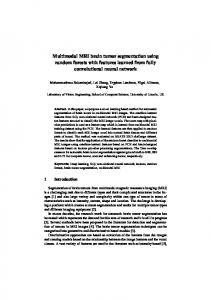
Figure 2.2: Non-brain tissue removal for sample slice (25th) from first dataset on T1-weighted scan: Raw image on the left and skull-stripped image on the right

50

50

100

100

150

150

200

200

50

100

150

200

50

100

150

200

Figure 2.3: Removing extremely high and low values for a sample slice (25th) from first dataset on T1-weighted inversion recovery scan: On the left raw image and on the right the image after applying this preprocessing step. (T1-IR shows the effect of this preprocessing step clearly since variation of the intensity values of this channel was significant) any voxels outside of the brain were mapped to zero as background. Fig. 2.2 shows the effect of this step for a sample slice. • Removing extreme high and low intensity values from training and testing dataset: Outlier intensity might have an adverse impact on the segmentation results. Therefore, 4th percentile and 96th percentile of each datasets were calculated as boundaries and all voxels below and above these calculated values were clipped off and mapped to derived boundaries. Fig. 2.3 shows how this step affected a sample slice. • Normalizing data : Since intensities from different channels within a patient and also intensities of same channels for different patients could have large variability, normalization is a critical step to be applied on data. Table 2.1 shows this variation for one sample training channel of dataset (after 5

applying previous preprocessing techniques). Therefore, in this project all images were normalized with zero mean and standard deviation of one. Table 2.1: Variation of intensity for different datasets (T1-weighted channel)

2.3

Dataset

Min.

Max.

Mean.

1 2 3 4 5

19 19 25 16 18

230 196 243 238 222

40.98 39.45 48.39 37.92 41.41

Feature Extraction

As the input of networks (both layers), features were extracted via two separate approaches. One set of features were conventional intensity-based and spatial-based features. Same features as [13] were extracted from images which are described as following: • Intensities of different channels (T1-weighted, T1-IR and T2-FLAIR) • The intensity after convolution with a Gaussian kernel with σ = 1, 2, 3 mm2 (both in 2D and 3D manner) • The gradient magnitude of the intensity after convolution with a Gaussian kernel with σ = 1, 2, 3 mm2 (both in 2D and 3D manner) • The Laplacian of the intensity after convolution with a Gaussian kernel with σ = 1, 2, 3 mm2 (both in 2D and 3D manner) • Spatial information of all voxels (x, y, z) which were divided to length, width, and height of the brain respectively. Other features such as Gabor filter bank, Haar features, histogram based features (e.g. histogram equalization and contrast-limited adaptive histogram equalization) were extracted from datasets. However, their impact on the results was not significant. Thus, at final implementation, they were not utilized. Moreover, T1-IR channel was not used as a direct feature since it had large variability which degraded the segmentation results. Totally, 32 features were extracted and used from this stage of the method. Another important set of features, used in this project as extra channels, was results from level set method which is described in next section. 6

2.4

Shape Context generation based on level set

In order to incorporate the shape prior into the machine learning framework a shapemodel guided level set method was used to generate preliminary segmentation masks of different brain structures [11], namely inner skull surface, brain ventricles, basal ganglia, cortical GM-WM surface and cortical GM-CSF surface. The distance maps of these segmented masks are then used as context information for the classifier training i.e. using the readout of these maps as additional features that are passed into the classifier. For segmenting the skull, ventricles and basal ganglia, conventional statistical shape models that were trained from the five training datasets were used. For segmenting the surfaces of the cortical GM, a skeleton-based shape model was used to guide the level set propagation. For more detail description of this methods, readers are referred to [11].

2.5

Classifier Training

Artificial Neural Networks were used as main learning algorithm of the proposed algorithm. Several ANN-based algorithms 2 including support vector machine (SVM), multi layer perceptron (MLP), radial basis function (RBF), learning vector quantization (LVQ) and convolutional neural networks (ConvNets) were implemented in the frame of this project. However, the results from MLP were relatively accurate and also training time was considerably shorter compared to other methods. Thus, this network was chosen for this project. The proposed network consisted of one hidden layer with 100 hidden nodes. The learning rule for updating weights was generalized delta rule which calculated the weight updates from output to input layer (error back-propagation) [14]. In the training phase, n × 10000 voxels were randomly selected from n training datasets within the brain region excluding the cerebellum and the brain stem. For each voxel, 37 features (32 image features + 5 context features) and the corresponding labels are passed into the ANN. The training label includes 6 classes, namely WML, WM, Cortical GM, basal ganglia,ventricles and CSF. The ANN training was set to stop after 1000 iterations. The output of second network contained the information of the voxel classes which were used for final segmentation as described in next section.

2.6

Image Segmentation and Post-processing

For segmenting the test dataset, all voxels are passed into the ANN, which in turn output the probabilities of the voxel belonging to those 6 classes. The voxel is 2

Thorough explanation about these networks can be found in appendix

7

assigned to the class that gives the highest probability. Networks were trained with six labeled classes, thus the network results also included six classes. However, these six classes had to be merged to form final three segmentation parts (i.e. WM, GM and CSF). The method for merging different classes can be found on [3].

2.7

A Variation of the Proposed Segmentation Framework

Auto-contexting is a popular approach to improve the segmentation accuracy of the image classifier that are trained using local patches. The principle of auto-contexting is to retrain a new classifier using the output of previous classifiers as additional features to the image features. To see whether auto-contexting will further improve the segmentation accuracy of the proposed method, an alternative processing pipeline was implemented as summarized in the part marked with dash lines in Fig. 2.1. In order to exploit the context information, outputs of the first network which were discriminative probability (or classification confidence) were convolved with Gaussian filters with kernel size of 0.5 mm and 1 mm and then sent to the second network as extra features along with all other obtained features. The structure of the second network was identical to that of the first one. This auto-texting layer can be repeated a number of times. In our project, we tested up to 2 auto-texting layers

2.8

Accuracy Analysis

Segmentation results were compared to ground truth based on Dice similarity index and absolute volume different (AVD) similarity index and 95th-percentile of the Hausdorff distance (HD) index [3]. While Dice coefficient indicates how the two masks overlap with each other, HD gives the largest distance between two contours. AVD on the other hand can indicate whether there is a systematic error with volume measurement. Background, cerebellum and the brain stem were excluded from validation.

8

Results

The proposed method was first tested on the 5 training datasets. For the shape context generation, the statistical shape models described in section 2.4 were generated using all 5 training datasets and applied to the 5 training datasets. While the ANN based voxel classification was tested using leave one out method. Table 3.2 shows comparison between three implemented methods. The results were drived using leave-one-out method for training datasets. As it is illustrated, MLP achieved better performance with acceptable training time. Therefore, this method was chosen as final choice of ANN structure. For SVM, 15 support vectors were trained and for CNN the same structure represented in Fig. A.6 was used (The results obtained presented for SVM and CNN in Table 3.2 were obtained without auto-context layer

Table 3.2: Comparison of differnt ANN-based algorithms Method MLP SVM CNN

Dice(%) Dice(%) Dice(%) Dice(%) Dice(%) ICV Brain CSF WM GM 98.09 98.09 98.09

95.19 94.94 90.01

84.64 83.73 76.94

87.68 87.17 77.33

84.86 84.32 67.00

For ANN training, the n × 10000 train samples are randomly selected from the training set. In order to investigate the randomness’s impact on the segmentation accuracy, the whole leave-one-out method was executed five times with exactly same parameters and structure, but with different random samples. The mean value and standard deviation of the variance of Dice index and ADV index are shown in Table 3.3.

9

Table 3.3: Investigating reliability of proposed method using MLP network

Structure

Mean variance Dice(%)

GM WM CSF Brain ICV

0.107 0.103 0.139 0.044 0.029

Mean Std.dev(%) variance AVD(%) 0.135 0.137 0.176 0.055 0.039

0.662 0.656 0.903 0.234 0.217

Std.dev(%) 0.898 0.827 1.11 0.292 0.255

In order to see the effect of exploiting shape features on results, one test was performed without shape features (only other 32 features) and another test was performed including shape features. Comparison of results between pure ANN, pure shape model level set and the combined method can be seen in Table 3.4. In addition, in Fig 3.4 misclassified pixels are shown for a sample slice for three different approaches which are level set method, ANN-based method and combination of both methods. Table 3.4: Effect of adding shape model. Method MLP level set MLP + level set

Dice(%) Dice(%) Dice(%) Dice(%) Dice(%) ICV Brain CSF WM GM 97.62 96.79 98.09

94.84 94.48 95.19

83.29 78.34 84.64

85.45 87.74 87.68

82.50 82.56 84.86

In order to investigate the effect of auto-context layer mentioned in section 2.7, three tests were performed. One without auto-context layer, one with one layer of auto-context and the final test with two layers of auto-context. The results are shown in Table. 3.5. Table 3.5: Investigating the effect of auto-context layers (Tests were performed with 700 iterations and 20000 training samples) Method Without Auto-context 1 Layer of Auto-context 2 layers of Auto-context

Dice(%) Dice(%) Dice(%) Dice(%) Dice(%) ICV Brain CSF WM GM 97.72 97.72 97.72

95.06 95.04 94.98

10

83.88 83.79 83.70

87.26 87.27 86.93

84.51 84.57 84.40

50

50

50

100

100

100

150

150

150

200

200

200

50

100

150

200

50

100

150

200

50

100

150

200

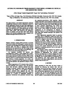
Figure 3.4: Misclassified voxels in 24th slice of 5th dataset. Results for level set is shown on the left, results for MLP is shown in middle and results for hybrid model is shown on the right image. The total number of misclassified voxels for this dataset was 138538, 71321 and 67507 for level set method, ANN method and hybrid approach respectively.

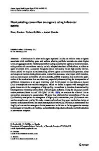
Fig. 3.5 shows final results after segmentation with proposed algorithms for three sample slices for visual inspection. The first row shows sample raw images which were used for feature extraction as input of the network. The second row shows the results of proposed segmentation method and third row shows the misclassified pixels in these three sample slices.

Table 3.6 shows the MRbrain image segmentation results for test datasets. The evaluation was performed by MRBrains13 challenge organizers who also provided the extensive comparison to other segmentation approaches on same datasets. The proposed method (STH in the table) was ranked 6th taking to account all segmentation scores and was ranked 2nd for segmenting brain tissue ( GM + WM )3 . Totally 35 teams participated in the challenge at the time of writing this report. In Table 3.6 the first three rows show the results of top three teams in the challenge respectively. The fourth row belongs to CMIV which used only shape model level set method. The final row represents the results for proposed method. According to Dice coefficient the worse accuracy differences between 1st rank and the proposed method is 0.71% as it is shown in the table.

3

For further details about ranks and score please visit: (http : //mrbrains13.isi.uu.nl/results.php)

11

50 100 150 200

50 100 150 200 50 100 150 200

50 100 150 200

50 100 150 200 50 100 150 200

50 100 150 200 50 100 150 200

50 100 150 200

50 100 150 200 50 100 150 200

50 100 150 200 50 100 150 200

50 100 150 200

50 100 150 200 50 100 150 200

50 100 150 200

50 100 150 200

Figure 3.5: Examples of segmentation results for three slices (10, 25, 35) for 5th dataset. First row shows the raw T1-weighted scan, second row shows the segmentation result from proposed method and the third row shows the misclassified pixeles in these three sample slices. ( Note: Cerebellum and brainstem were removed manually using the ground truth) Table 3.6: The performance comparison on MR brain challenge. Structure

GM

WM

CSF

DC(%)

HD(mm)

AVD(%)

DC(%)

HD(mm)

AVD(%)

DC(%)

HD(mm)

AVD(%)

FBI/LMB

85.44

1.58

6.60

88.86

1.95

6.47

83.47

2.22

8.63

LSTM2

84.89

1.67

6.35

88.53

2.07

5.93

83.05

2.30

7.17

IDSIA

84.82

1.70

6.77

88.33

2.08

7.05

83.72

2.14

7.09

CMIV

82.56

2.83

7.63

87.74

2.46

7.15

78.34

3.09

15.63

STH

84.78

1.71

6.02

88.47

2.36

7.66

82.76

2.32

6.73

12

All experiments were performed on a desktop computer with NVIDIA GTX 980 4GB , 32 GB installed memory and Intel Xeon E5-2630 2.40 GHz CPU. Main implementation of the algorithm was done with MATLAB (version 2016a). The runtime of implemented algorithm for training networks and testing on a volume was 14 minutes approximately (around 5 minutes for ANN and around 9 minutes for level set method).

13

Discussion The main contribution of this study is proposing a new segmentation algorithm which incorporates the shape prior into the machine learning framework by combining an ANN-based learning algorithm and a shape model based level set method. This hybrid solution delivers better performance compared to either of them individually (c.f. Table 3.4 and Table 3.6). When compared with ANN using only image feature, adding the shape prior knowledge helped the algorithm to recognize the basal ganglia areas inside the brain. And when compared with the pure statistical shape guided level set implementation, the improvement is more on the edges of the brain structures. Notice the model based level set method uses only the intensity of the T1 image to perform the segmentation, while ANN uses 32 image features of all 3 MRI sequences. Also when compared to auto context models which were used [4, 15] (rank 4th and 5th in challenge), the shape context information seems to be at least as good as multi-iteration auto-contexting (see Table 3.6), but the proposed method needs just a single iteration. In fact, in our experiments, adding more auto-contexting iterations do not improve the segmentation accuracy further. As it can be seen from in Fig. 3.5, most of the segmentation errors within the brain occurred in the border of different brain tissues, where inter-observer variation of the manual delineation could also be high. However, a single ground truth segmentation was generated for each testing data through consensus sessions so the inter-observer variation of the segmentation accuracy is unavailable. Yet, when comparing the Dice coefficient of the top 3 methods for each brain structure, the variation is mostly below 1%. From our experiments, skull stripping is a prominent source of error. To investigate how much it could affect the results, one test was executed with the proposed skull stripping algorithm and one test was executed by using manual segmentation for skull striping (i.e. perfect mask). The results of this approach suggests that approximately 2% of the error for segmenting ICV and 5% of the error for segmenting CSF was related to skull stripping. It had very small effect on GM segmentation and almost no effect on WM segmentation. Another challenge of processing the MR brain segmentation challenge data is to handle the WML class (MS lesion) properly. While running the leave one out test, we noticed for one of the dataset (patient 2), Dice index of WM was considerably smaller 15

compared to other datasets. After further investigation on this special dataset, it was revealed that this 3D volume consisted of a greater fraction of WML compared to other datasets. This suggests, for the training, there should be enough number of random sample within the WML regions to ensure the correct classification of this special type. As shown in Table 3.3, the results are reproducible and the segmentation accuracy changes only slightly when using different sets of randomly selected training samples. Increasing size of training data can lead to even smaller standard deviation with the cost of expensive calculations. In this project we also tested different ANN settings. As Table 3.2 suggests, MLP and SVM produce comparable results, but the former is much faster to train. Deep learning approach using CNN was also tested, however, the current implementation delivers inferior results than those of conventional ANN methods, which suggests more tuning is needed. However, due to the limited time, this approach is not further investigated. Many possible extensions could be considered as further development of this study. Principle component analysis (PCA) can be applied on features to firstly reduce size of features and probably increase the performance. This step could be highly beneficial in case of extracting more features. However, there would be no guarantee for further improvement of the result if more features are extracted. In addition, using the results from other conventional methods could affect the results and create a new hybrid system. Finally, cross validation could be performed on training data for determining the best parameters of the network which needs sufficient time and also a powerful system for running the program.

16

Conclusion In this project, a fully automatic method has been proposed which incorporates the shape prior into the machine learning framework by combining an ANN-based learning algorithm and a shape model based level set method. Results for segmenting WM, GM and CSF of the brain performed using proposed method were relatively accurate with acceptable standard deviation while the training and testing time were considerably shorter compared to other methods . Further investigation is needed for developing current method to improve the accuracy. Moreover, the generalization power of the proposed algorithm in other field of medical imaging segmentation is open for further studies.

17

Appendix A Appendix: The state of the art methods for medical image segmentation based on machine learning This chapter includes brief theoretical background about medical image segmentation and explanation about the most new techniques for brain image segmentation with learning based approaches. It also describes the common preprocessing and post processing methods for MRI scans to enhance the accuracy and efficiency of final segmentation results.

A.1

Background

Image segmentation refers to techniques for partitioning digital images to multiple homogeneous and non-overlapping areas which represents the image in a way to be analyzed visually or computationally for different applications. In medical applications, image segmentation could be highly beneficial for studying anatomical structures of the body, determining region of interests (e.g locating tumors), measuring tissue volume, surgery planning before radiation therapy, image-guided interventions, post-surgical assessment, virtual surgery simulation, etc [2, 16, 17]. Among different applications, brain image segmentation is one the most important diagnostic tools for detecting and predicting many brain related diseases and abnormalities such as small vessel disease, Alzheimer disease, dementia, focal epilepsy, Parkinson and also for analyzing brain development [1–3]. Segmented areas or different classes on brain scan could include different tissue types. However, the three most important parts of the brain are usually gray matter (GM), white matter (WM) and Cerebrospinal fluid (CSF). Fig. A.1 shows theses different areas on two 19

Figure A.1: Two sample T1-weighted MR images which are manually segmented by three experts (Data adapted from http://mrbrains13.isi.uu.nl/).(Left image from middle part of the brain and right image from lower part of the brain). The segmented areas are written on the images as area 0 is background, area 1 is Cortical gray matter, area 2 is Basal ganglia, area 3 is White matter, area 4 is White matter lesions, area 5 is Cerebrospinal fluid in the extracerebral space, area 6 is Ventricles, area 7 is Cerebellum and finally area 8 is Brainstem. In case of segmenting to only four areas (background, GM, WM and CSF) area 1 and 2 can be merged as GM, areas 3 and 4 can be merged as WM and areas 5 and 6 can be merged as CSF. T1-weighted sample slices from 3D MR scans. Magnetic resonance imaging (MRI) and computed tomography (CT) are the most common non-invasive methods for analyzing the anatomical structure of the brain [17]. While CT is usually used for detecting bleeding, brain damage and skull fractures in patients, MRI is preferable for brain image segmentation application. MR in general has excellent contrast and signal to noise ratio (SNR) for soft tissue imaging and also it is more sensitive for detecting brain diseases in early stage for instance for detecting tumors or white matter diseases. In addition, it is less harmful compared to CT [17]. By using different pulse sequences and changing imaging parameters in MRI which are related to longitudinal relaxation time (T1), and transverse relaxation time (T2) and also signal intensities, different image types could be acquired. Each of these image types with different level of contrast could have applications for analyzing specific tissue in brain. Common MR imaging acquisition protocols are T1- weighted scans, T2-weighted scans, proton density (PD), T1-weighted inversion recovery scans and fluid attenuated inversion recovery (FLAIR) scans [3, 17].

A.2

Brain Image Segmentation

Currently, the most accurate method for segmenting MR scans is manual segmentation. Manual segmentation is usually performed in dark room with optimal viewing 20

condition by expert physicians and clinicians [3]. Indeed, most of the time even for evaluation of other segmenting methods, their results will be compared with manually segmented images as ground truth. Physical or computational phantoms are also used for validating segmentation methods, but usually they do not provide a realistic representation of anatomical structures. Basically, brain atlases are formed by these manually manipulated images [18]. It should be noted that manual segmentation is a complex and tedious task for clinicians [1]. Manual segmentation is typically performed slice by slice even for 3D volume. Therefore, manual segmentation, although accurate, is very time consuming. In addition, this method is subjective (e.g. related to experience and skill of the operator) and very difficult to be reproduced [1], [5]. A number of softwares such as ITK-Snap [19] show different views of the brain (i.e. sagittal, coronal, and axial). Thus, it could be very helpful for experts to conduct better and more accurate manual delineation. Many other semi-automatic and non-automatic computer aided algorithm are proposed in the literature for brain image segmentation including intensity based methods (including thresholding, region growing), atlas-based methods (using prior knowledge), contour-based methods (including active contours and surfaces, and multiphase active contours) [1]. The common problem of all these methods is accuracy. They may perform well for specific data, but they are not reliable for another dataset. However, they could be used as part of learning approaches in automatic segmentation methods [17]. Indeed, there are new approaches that try to combine different methods to avoid their disadvantages and limitations and at the same time get the best out of each of them. They are generally called “Hybrid segmentation methods” [1]. Because of all mentioned problems, the need for fully automatic and reliable methods for brain image segmentation has emerged. Although, automatic methods have different performance (e.g. in terms of complexity, accuracy, computational speed, etc), most of them are based on learning approaches and share a common structure. The main scheme of these approaches is shown in Fig. A.2 . As Fig. A.2 shows the main components of the flowchart are: • Data • Pre-processing • Learning approaches based on feature extraction or Deep learning 21

Figure A.2: Generic flow chart of automatic segmentation algorithms • Post-processing • Validation of results In the following parts of this chapter, each of these sections will be described and the state of the art methods for each part will be explained.

A.2.1

Data

Usually, MR scans are presented as 2D images (pixel-based) or 3D volume (voxelbased). The value of each pixel or voxel represents the intensity of signal which is related to magnetic resonance characteristics of corresponding tissue. Actual pixel/voxel size depends on parameters such as imaging parameters, magnet strength, etc, but usually it is around 1-2mm [1]. It is recommended to use common and reliable data (e.g from previous challenges and online sources such as Internet Brain Segmentation Repository (IBRS) [20], MRBrainS [3] and Alzheimer’s Disease Neuroimaging Initiative (ADNI) [21]). These datasets provide manual segmented images as ground truth which can be used for both training and evaluation of segmentation algorithms. In addition, using these datasets makes it possible to compare results with other implemented segmentation algorithms on the same data. In order to estimate the segmentation method error at the end, data are divided to two groups. One group for training the segmentation algorithms and the other group for testing the algorithms. Since data are valuable and sometimes insufficient, 22

advance methods are introduced for dividing train and test data including holdout, re-substitution, cross-validation, leave-one-out and boot-strapping.

A.2.2

Preprocessing

Preprocessing is one the most important parts that must be done before applying segmentation algorithms. Different artifacts can corrupt MRI scans such as image noise, motion artifact, partial volume effect and bias field effect. One should remove these artifacts in order to improve the final segmentation results. Beside these artifacts, non brain tissue should be removed from images since it degraded segmentation result dramatically [1]. Different methods for noise reduction in MRI scan can be applied. Some MRI de-noising methods are linear filtering methods, nonlinear filtering methods, Markov random field (MRF) models and wavelet transform [2]. Bias field effect (also called intensity inhomogeneity) refers to smooth signal intensity variation within the same tissue. This artifact arises from spatial inhomogeneity of the MRI device. This artifact is correlated with magnetic field (negligible in 0.5T and high in 3T magnetic field) [1]. This artifacts can be modeled as low-frequency component and can be removed by low-pass filtering [22]. However, low-pass filtering may also remove low frequency components in true image. Therefore, more advanced algorithms are proposed in literature for removing that such as minimizing the image entropy [23], maximizing the high-frequency components of the image [24]. Also some software such as SPM8 [25] and FSL [26] could do this preprocessing step. Another preprocessing technique specially in case of using multi dataset or multimodal images (e.g., MRI, CT, PET, and SPECT), is registration. Registration is the process of finding the transformation between images with corresponding features and aligning images spatially. Registration is crucially important when there is motion artifact (e.g patient movement) in the images. Rigid and affine transformation are two typical methods for performing registration [27]. In addition some software such as Elastix [28] can be used for image registration. It should be noted that in general registration task becomes more challenging when brain images include lesions or diseases since it is more difficult to align healthy and abnormal tissues [1]. Partial volume effect (PVE) is another artifact that degrades the segmentation result. It refers to loss of small tissue regions because of the poor resolution of the MRI scanner [1]. Indeed when two or more tissues affect one pixel or voxel, the result image will be blurred specially at the boundaries between tissues [17]. One 23

Figure A.3: Histogram of a T1-Weighted MRI of an adult brain (Adapted from http://www.hindawi.com/journals/cmmm/2015/450341/)

good solution to deal with this problem is soft segmentation which means each pixel can belong to several classes according to specific criteria (see B.4) [17].

As mentioned previously another important step in preprocessing is removing non brain tissue. Non brain tissues include skull, scalp, dura mater, fat, skin, muscles, eyes and bones [1]. One way for removing non brain tissue is using mask which is generated according to prior knowledge (e.g. brain atlases) [29]. However, this method is not very precise. An alternative method is using brain extraction tools (BET) which is part of free FSL software [26]. This software tries to find the center of gravity of the brain and then inflate the sphere until it reaches the boundary. It has shown acceptable performance for T1-weighted and T2-weighted images.

Based on need and input images, other preprocessing steps such as normalization (usually with zero mean and unit standard deviation) and range-scaling can be applied on data before feature extraction and classification [30].

Hopefully, after all preprocessing steps, histogram of the images should have three main peaks which represents WM, GM and CSF. Fig. A.3 shows a sample preprocessed T1 MR histogram for an adult [1] (Peaks are not that separable for Neonates). As Fig. A.3 shows, there is overlap between different parts and overlap between GM and WM is more than the overlap between GM and CSF. However, researches show adding additional MRI sequences (e.g T2-weighted) can be helpful and eventually improve segmentation results [1]. 24

A.2.3

Features

Most of learning based methods for image segmentation are based on features that are extracted from images. Therefore, it is worthy to know more about these features. Generally, features are extracted from images by numerical measurements and with aid of them it is possible to discriminate between regions of interest and their background. Appropriate feature selection and feature extraction plays important role in final segmentation results [1]. One set of conventional features that are used for MRI classification are statistical features. Statistical features are based on first and second order statistics of intensities in images. First order statistical features can be derived from image histogram and includes intensity, mean, median, and standard deviation (SD) of images. First order features are useful for image segmentation when background and object of interests have different intensities in large scale [1]. Second order statistical features are usually used for describing image texture and can be extracted from Co-occurrence matrix of images [31]. Energy, contrast, entropy and correlation are some of the features that are used as second order features for brain image segmentation [32]. First and second statistical features are usually called appearance features in literature. Another popular feature for image segmentation is edge (i.e boundaries in the image when there is a sharp change in intensities value) [1]. Edges in general are sensitive to noise so de-noising must be performed in preprocessing stage for proper edge detection. Edge detection is usually based on gradient (derivative) function. It could be first order (e.g. Prewitt, Sobel, Roberts) or second order derivative (e.g. Laplacian). In literature, Gaussian-scaled gradient magnitude and Gaussianscaled laplacian of intensity have been used along with intensity and Gaussianscaled intensity for brain image segmentation [30]. Also more advanced methods are proposed in literature for edge detection such as phase congruency method [33] and Canny edge detection [34]. Gabor filter is another linear filter for edge detection. This filter is sensitive to orientation and frequency in the edges and it has been found particularly appropriate for for texture discrimination in the image. Gabor filters have been used for brain image segmentation along with other features [35]. Moreover, Haar-like features could be used for medical image segmentation. They have been used successfully for face recognition in literature [36]. In this method adjacent rectangular regions are considered in certain locations in the detection window. Then, sum of pixel intensities in these rectangular areas are calculated and the difference between these sums are derived. The difference could be used to differentiate different areas in the original image. Since Haar-like feature is a weak classifier a large number of Haar-like features are needed to segment the image 25

properly. This feature has been used for brain image segmentation in literature [35]. Spatial information (i.e. x, y, z coordinates of voxels) also can be used as an extra features. However, this feature should be used carefully if images are not aligned properly. Some studies have shown the impact of using these features on improving brain image segmentation results [30].

A.2.4

Learning approaches

Probably, the most important part of the flowchart in Fig. A.2, is segmentation method. Segmenting MRI scans could be very complicated task since images are imperfect and corrupted with different kind of artifacts (even after preprocessing). Therefore, many image processing techniques have been proposed in literature for medical image segmentation. However, between them learning based approaches (considered as automatic segmentation methods in this report) have shown better performance. In general, they can be divided to supervised learning approaches (i.e. training with labeled data as ground truth) and unsupervised learning approaches (i.e. train themselves with unlabeled input data). In the following, the most important techniques with acceptable performance are described briefly. KNN Classifier: In nearest neighbor classifier each element (pixel or voxel) is classified as the same class of training datum with closest intensity. K-nearest classifier is the generalized version which each element is classified based on majority votes of the closest training data. This method was used in literature for MRI brain segmentation [37], [38]. In those studies, beside intensity, spatial localization of brain structure was used as an additional feature. Bayesian Classifier: This classifier tries to model the relationship between feature sets and class variables and then use this model to estimate the class of unknown samples [39]. Expectation maximization (EM) segmentation methods are based on Bayesian classifier and have been used in many software packages such as SPM [40], FreeSurfer [41] and FAST [42]. K-means Clustering or Hard C-means: This is an unsupervised iterative method which starts segmentation by putting input data to K different classes. Then in each iteration, it computes the mean intensity (called centroid) for each class and classifies each element into the closest centroid. K-means clustering is known as hard classifier since it force each element to belong 26

Figure A.4: Generic topology of ANN. Wij shows the weights between input and hidden layer and Wjk shows the weights between hidden and output layer. ANN could have more than one hidden layer to a class in each iteration [43]. Soft version of this method is Fuzzy C-means Clustering (FCM) [44] which let the elements belong to multiple classes based on certain membership value. Artificial Neural Network Approaches: There are some approaches for image segmentation with promising results that uses artificial neural network (ANN)1 in their main structures. Generally, these networks consists of input layer (the number of input nodes shows the feature dimension that are extracted from MR images), nodes (building block of the network), activation functions (which affects output of each node), learning rule (depends on the algorithms it could change such as perceptron learning rule, delta rule, generalized delta rule and Kohonen learning rule), topology (connection between different nodes, input and output layer) and output layer (only for supervised approaches). Fig. A.4 shows the topology of ANN. Here, most important algorithms of ANN that can be used for segmentation are explained. • Multi Layer Perceptron (MLP): MLP is a feed-forward network with general structure as it is shown in Fig. A.4. It is combined of several linear classifiers (each perceptron) that can be together used for non linear classification problem. The weights of network are randomly initiated at first and then in each iteration they will be updated according to generalized delta rule in order to minimize the error function (difference between network output 1

In this report all methods which use artificial neurons (nodes) as their building blocks are considered as ANN

27

Figure A.5: Generic Architecture of RBF network for two classes classification.µ1 , µ2 ...µk are activation functions based on euclidean distance. and real output). The method for updating is called back propagation (BP) since updating weights are performed from output layer toward input layer. This method uses gradient descend for minimizing the error function so it may get stuck in local minima [14]. For implementing this method some parameters has to be tuned such as number of nodes in hidden layer, number of hidden layers, number of iterations (trade off between bias and variance), etc. For tuning these parameters some proposed solutions are cross validation and early stopping rule [14, 32]. This method has been used in literature for brain image segmentation [32] and also outdoor image segmentation [45] with promising results.

• Radial Basis Function (RBF): RBFs are sets of networks that try to map nonlinear input space to linear feature space and then classify it linearly [14]. For mapping, euclidean distance is used in activation functions. Like MLP network, here again gradient descend approach is used for minimizing error function. The generic architecture of RBF is shown in Fig. A.5 . RBF network can be used for brain image segmentation alone [46] or as part of other approaches. For instance SVM, SOM and LVQ use RBF neurons for classification.

• Support Vector Machine (SVM): SVM is a nonlinear binary classifier that can be used for supervised learning. It takes input labeled data from two classes and updates the network for classifying unlabeled data [47]. The weights in this network are updated in order to optimize two terms: maximize the border around decision function and minimize the number of training 28

samples that are wrongly classified. Further information about this algorithm can be found in [48]. Basically SVM is a binary classifier, but it can be used for multi classification by using some approaches such as one-versus-one method [30]. This method showed promising result for brain image segmentation, but computationally expensive [30]. For reducing the training and testing complexity, the size of original dataset can be reduced by using certain properties e.g. discrete wavelet transform [47].

• Self Organizing Maps (SOM): This is an unsupervised clustering method that was introduced by Kohonen in 1982 for the first time. SOM network consists of input layer and competitive layer (hidden layer in Fig. A.4). Number of nodes in input layer shows number of features and number of nodes in competitive layer shows number of classes (e.g. four nodes for segmenting background, WM, GM and CSF in brain MRI scans). The algorithms can be divided to three phases. Competitive, cooperation and adaptive phase. In Competitive phase, for each input sample, one neuron will be specified as winner neuron. This node has the minimum euclidean distance from the input data. In cooperation phase neighbors of the winning neuron are specified. Generally, neighborhood is specified by a Gaussian function (winning node in the center of Gaussian function and other nodes will be distributed on Gaussian function). Final phase is adaption phase which weights of winning node will be updated. Weights of the neighbor nodes also will be updated, but with less strength (according to Gaussian distribution in cooperation phase). Updating weights is done based on Kohonen learning rule and move the winning node and its neighbors toward the input data. In the other word, SOM network learn the distribution and topology of input data in each iteration and finally classify the input data to different clusters [2]. This method has been used for image segmentation in literature for instance for tumor detection [49].

• Learning Vector Quantization (LVQ): This method can be considered as supervised version of SOM. LVQ network consists of three layers: input layer, competitive layer and output layer. In competitive layer, input data are classified corresponding to SOM method. Thus, here again the winner neuron is specified based on the euclidean distance between the node and input data and the weights of winning node will be updated. The output layer maps the competitive layer classes to target classes. Indeed, the learning process in each iteration in LVQ method is related to updating winner node weights. When the winning node is determined by the competitive layer, then it will be checked if it is correctly classified (according to labeled training data). If it is classified correctly, the weights will be updated to move it closer to 29

input data and if it is wrongly classified, then it moves away from the input data [2]. Several algorithms are proposed in the literature for LVQ network with slight implementation differences. LVQ1, QLVQ, LVQ2.1 and LVQ 3 are some of these learning approaches. Practical experiences show that it is good to initiate the network with LVQ1 and then switch to other algorithms (e.g. LVQ2.1) in further iterations. Deep Learning: Deep learning is a relatively new branch in machine learning which tries to model high-dimensional input data by multilayer processing neural layers [50]. This approach consists of many architectures, but one which has high potential for image recognition is convolutional neural networks (CNN or ConvNet). For image segmentation, CNN analyses the neighborhood around each voxel (pixel) and tries to classify it. In CNN, there is no need for feature extraction and this is the main difference between CNN and other learning approaches. Instead, in CNN middle layers consist of kernels (some already established filter banks) which are convolved with input data. Generally, for classifying each element (pixel or voxel) in CNN, first a small patch from the original image is chosen with the desired element (the pixel or voxel to be classified) in center of patch. Then this patch will be convolved with kernels in middle layer or layers and create feature maps in output. Usually, the final layer is fully connected conventional MLP which creates the final classification output. In literature, CNN has been used for anatomical brain segmentation with promising results [51–53] . Fig. A.6 shows one of the implemented CNN architecture for brain image segmentation to GM, WM, CSF and Background [53].

A.2.5

Post-processing

Different post-processing techniques could be applied on classifier output. The postprocessing part mainly depends on the techniques that are used in previous parts. For instance, if 2D slices were used for segmentation, then combing these slices to form 3D volume could be a post-processing task [1]. Another post processing step could be fusing voxel values of segmented result to reduce the number of classes (see Fig. A.1)

A.2.6

Validation methods

A common problem for medical image segmentation is quantitative comparison and validation. For proper comparison, a gold standard or ground truth is needed. Unfortunately, there is no real ground truth for in vivo brain analysis. Thus, ground truth is made by one or more experts after image acquisition as manual segmentation. As mentioned earlier, this method needs to be critically considered, but so far 30

Figure A.6: Brain image segmentation using CNN architecture applied on IBRS data [53]. In left side, a patch is chosen from the 3D volume (with size of 9 × 9 × 5). Then it convolved with filter banks in middle layers (layer one consist of 20 feature maps and layer 2 consists of 60 feature maps). The output of layer two is send to two fully connected hidden layers which finally classified the voxel. (Adapted from www.diva-portal.org/smash/record.jsf?pid=diva2%3A814233&dswid=6260) it is the most accurate approach for evaluation of segmentation algorithms. For quantifying the overlap between manual segmentation and different segmentation methods, several measures are proposed in the literature. One of the most popular similarity indexes which determines the spatial overlap is Dice similarity index (DI). It can be be calculated as following: T 2|Ai Bi | (A.1) DI% = |Ai | + |Bi | where i stand for tissue types (e.g. WM, GM, CSF), A stands for manual segmentation (ground truth) and B for MRI segmentation algorithm. It has the range from 0 (the worst result) to 100 (the best result if A and B are completely identical). Another similarity index (again for spatial overlap) which has been used in literature [32] is Jaccard similarity index (also called as Tanimoto coefficient) which can be derived as following: T T |Ai Bi | |Ai Bi | S T JI% = = (A.2) |Ai Bi | |Ai | + |Bi | − |Ai Bi | where i, A and B have the same definition as in Dice index. Hausdorff distance also can be used as validation methods which is sensitive to segmentation boundaries. Hausdorff distance measures the distance of two subsets of a metric space. Conventional Hausdorff distance is very sensitive to outliers so 31

95th-percentile of the Hausdorff distance could be used instead. It can be calculated as following: th H95 (A, G) = Ka∈A min||g − a|| (A.3) th where Ka∈A is the kth ranked minimum Euclidean distance, A is set of boundaries points of segmentation result and G is set of boundaries points of ground truth.

A simpler validation method [3] is absolute volumetric differences measurement which is defined as: |Va − Vg | × 100 (A.4) AV D% = |Vg | where Va is volume of segmentation result and Vg is volume of manual segmentation. All these measurement can be used for different brain structure including GM, WM, CSF, brain (GM+WM) and intracranial volume (GM+WM+CSF).

32

Bibliography [1] I. Despotovi´c, B. Goossens, W. Philips, I. D. T, B. Goossens, and W. Philips, “MRI Segmentation of the Human Brain: Challenges, Methods, and Applications,” Computational and Mathematical Methods in Medicine, vol. 2015, 2015. [2] M. A. Balafar, A. R. Ramli, M. I. Saripan, and S. Mashohor, “Review of Brain MRI Image Segmentation Methods,” Artificial Intelligence Review, vol. 33, no. 3, pp. 261–274, 2010. [3] A. Mendrik, K. Vincken, H. Kuijf, M. Breeuwer, W. Bouvy, J. de Bresser, A. Alansary, M. de Bruijne, A. Carass, A. El-Baz, A. Jog, R. Katyal, A. Khan, F. van der Lijn, Q. Mahmood, R. Mukherjee, A. van Opbroek, S. Paneri, S. Pereira, M. Persson, M. Rajchl, D. Sarikaya, O. Smedby, C. Silva, H. Vrooman, S. Vyas, C. Wang, L. Zhao, G. Biessels, and M. Viergever, “MRBrainS Challenge: Online Evaluation Framework for Brain Image Segmentation in 3T MRI Scans,” Computat Intellig Neuroscience, 2015. [4] P. Moeskops, M. A. Viergever, M. J. N. L. Benders, and I. Iˇsgum, “Evaluation of an automatic brain segmentation method developed for neonates on adult MR brain images,” in SPIE Medical Imaging. International Society for Optics and Photonics, 2015, p. 941315. [5] S. Damangir, “Segmentation of White Matter Lesions – Using Multispectral MRI and Cascade of Support Vector Machines with Active Learning.” Master Thesis, KTH, School of Computer Science and Communication (CSC), 2011. [6] R. M. Haralick and L. G. Shapiro, “Image segmentation techniques,” Computer vision, graphics, and image processing, vol. 29, no. 1, pp. 100–132, 1985. [7] K. M. Pohl, “Prior information for brain parcellation,” Doctoral Dissertation, Harvard Medical School, 2005. [8] E. D’Agostino, F. Maes, D. Vandermeulen, and P. Suetens, “Non-rigid atlasto-image registration by minimization of class-conditional image entropy,” in Medical Image Computing and Computer-Assisted Intervention–MICCAI 2004. Springer, 2004, pp. 745–753. 33

[9] T. F. Chan and L. A. Vese, “Active contours without edges,” Image processing, IEEE transactions on, vol. 10, no. 2, pp. 266–277, 2001. ¨ Smedby, “Fast level-set based image segmentation [10] C. Wang, H. Frimmel, and O. using coherent propagation,” Medical physics, vol. 41, no. 7, p. 73501, 2014. ¨ Smedby, “Fully automatic brain segmentation using model[11] C. Wang and O. guided level sets and skeleton-based models,” Proceedings of the MICCAI Grand Challenge on MR Brain Image Segmentation (MRBrainS’13), 2013. [12] T. S. Yoo, M. J. Ackerman, W. E. Lorensen, W. Schroeder, V. Chalana, S. Aylward, D. Metaxas, and R. Whitaker, “Engineering and algorithm design for an image processing API: a technical report on ITK-the insight toolkit,” Studies in health technology and informatics, pp. 586–592, 2002. [13] A. V. Opbroek, F. V. D. Lijn, M. D. Bruijne, A. van Opbroek, F. van der Lijn, and M. de Bruijne, “Automated brain-tissue segmentation by multi-feature SVM classification,” Bigr.Nl, 2013. [Online]. Available: http://www.bigr.nl/files/publications/972 MRBpaper.pdf [14] S. Marsland, Machine Learning: an Algorithmic Perspective. CRC press, 2015. [15] L. Wang, Y. Gao, F. Shi, G. Li, J. H. Gilmore, W. Lin, and D. Shen, “LINKS: Learning-based multi-source IntegratioN frameworK for Segmentation of infant brain images,” NeuroImage, vol. 108, pp. 160–172, 2015. [16] Linda G. Shapiro; George C. Stockman;, Computer Vision, 1st ed. New Jersey: New Jersey, Prentice-Hall, 2001. [17] N. Sharma and L. M. Aggarwal, “Automated Medical Image Segmentation Techniques,” Journal of Medical Physics / Association of Medical Physicists of India, vol. 35, no. 1, pp. 3–14, apr 2010. [18] S. Egmentation, D. L. Pham, C. Xu, and J. L. Prince, “Current Methods in Medical Image Segmentation,” Annual Review of Biomedical Engineering, vol. 2, no. 1, pp. 315–337, 2000. [19] P. A. Yushkevich, J. Piven, H. C. Hazlett, R. G. Smith, S. Ho, J. C. Gee, and G. Gerig, “User-guided 3D Active Contour Segmentation of Anatomical Structures: Significantly Improved Efficiency and Reliability,” NeuroImage, vol. 31, no. 3, pp. 1116–1128, jul 2006. [20] IBRS, “IBRS,”The Internet Brain Segmentation Repository’,” 2013. [Online]. Available: http://www.nitrc.org/projects/ibsr 34

[21] C. R. Jack, M. A. Bernstein, N. C. Fox, P. Thompson, G. Alexander, D. Harvey, B. Borowski, P. J. Britson, J. L Whitwell, and C. Ward, “The Alzheimer’s Disease Neuroimaging Initiative (ADNI): MRI Methods,” Journal of Magnetic Resonance Imaging, vol. 27, no. 4, pp. 685–691, 2008. [22] M. S. Cohen, R. M. DuBois, and M. M. Zeineh, “Rapid and Effective Correction of RF Inhomogeneity for High Field Magnetic Resonance Imaging,” Human Brain Mapping, vol. 10, no. 4, pp. 204–211, 2000. [23] J.-F. Mangin, “Entropy Minimization for Automatic Correction of Intensity Nonuniformity,” in Mathematical Methods in Biomedical Image Analysis, 2000. Proceedings. IEEE Workshop on. IEEE, 2000, pp. 162–169. [24] J. G. Sled, A. P. Zijdenbos, and A. C. Evans, “A Nonparametric Method for Automatic Correction of Intensity Nonuniformity in MRI Data,” Medical Imaging, IEEE Transactions on, vol. 17, no. 1, pp. 87–97, 1998. [25] W. D. Penny, K. J. Friston, J. T. Ashburner, S. J. Kiebel, and T. E. Nichols, Statistical Parametric Mapping: The Analysis of Functional Brain Images. Academic press, 2011. [26] M. Jenkinson, C. F. Beckmann, T. E. J. Behrens, M. W. Woolrich, and S. M. Smith, “FSL,” Neuroimage, vol. 62, no. 2, pp. 782–790, 2012. [27] D. L. G. Hill, P. G. Batchelor, M. Holden, and D. J. Hawkes, “Medical Image Registration,” Physics in Medicine and Biology, vol. 46, no. 3, p. R1, 2001. [28] S. Klein, M. Staring, K. Murphy, M. A. Viergever, and J. P. W. Pluim, “Elastix: a Toolbox for Intensity-Based Medical Image Registration,” Medical Imaging, IEEE Transactions on, vol. 29, no. 1, pp. 196–205, 2010. [29] H. Xue, L. Srinivasan, S. Jiang, M. Rutherford, A. D. Edwards, D. Rueckert, and J. V. Hajnal, “Automatic Segmentation and Reconstruction of the Cortex from Neonatal MRI,” Neuroimage, vol. 38, no. 3, pp. 461–477, 2007. [30] A. van Opbroek, F. van der Lijn, M. de Bruijne, A. V. Opbroek, F. V. D. Lijn, and M. D. Bruijne, “Automated Brain-Tissue Segmentation by Multi-Feature SVM Classification,” Bigr.Nl, 2013. [31] R. M. Haralick, K. Shanmugam, and I. H. Dinstein, “Textural Features for Image Classification,” Systems, Man and Cybernetics, IEEE Transactions on, no. 6, pp. 610–621, 1973. [32] S. Amiri, M. M. Movahedi, K. Kazemi, and H. Parsaei, “An Automated MR Image Segmentation System Using Multi-layer Perceptron Neural Network,” Journal of Biomedical Physics & Engineering, vol. 3, no. 4, p. 115, 2013. 35

[33] P. Kovesi, “Edges Are not Just Steps,” in Proceedings of the Fifth Asian Conference on Computer Vision, 2002, pp. 822–827. [34] J. Canny, “A Computational Approach to Edge Detection,” pp. 679–698, 1986. [35] Z. Tu and X. Bai, “Auto-Context and Its Application to High-Level Vision Tasks and 3d Brain Image Segmentation,” Pattern Analysis and Machine Intelligence, IEEE Transactions on, vol. 32, no. 10, pp. 1744–1757, 2010. [36] P. Viola and M. Jones, “Rapid object detection using a boosted cascade of simple features,” in Computer Vision and Pattern Recognition, 2001. CVPR 2001. Proceedings of the 2001 IEEE Computer Society Conference on, vol. 1. IEEE, 2001, pp. I–511. [37] S. K. Warfield, M. Kaus, F. A. Jolesz, and R. Kikinis, “Adaptive, Template Moderated, Spatially Varying Statistical Classification,” Medical Image Analysis, vol. 4, no. 1, pp. 43–55, 2000. [38] H. A. Vrooman, C. A. Cocosco, F. van der Lijn, R. Stokking, M. A. Ikram, M. W. Vernooij, M. M. B. Breteler, and W. J. Niessen, “Multi-Spectral Brain Tissue Segmentation Using Automatically Trained k-Nearest-Neighbor Classification,” Neuroimage, vol. 37, no. 1, pp. 71–81, 2007. [39] W. M. Wells III, W. E. L. Grimson, R. Kikinis, and F. A. Jolesz, “Adaptive Segmentation of MRI Data,” Medical Imaging, IEEE Transactions on, vol. 15, no. 4, pp. 429–442, 1996. [40] J. Ashburner and K. J. Friston, “Unified Segmentation,” Neuroimage, vol. 26, no. 3, pp. 839–851, 2005. [41] B. Fischl, D. H. Salat, E. Busa, M. Albert, M. Dieterich, C. Haselgrove, A. Van Der Kouwe, R. Killiany, D. Kennedy, and S. Klaveness, “Whole Brain Segmentation: Automated Labeling of Neuroanatomical Structures in the Human Brain,” Neuron, vol. 33, no. 3, pp. 341–355, 2002. [42] Y. Zhang, M. Brady, and S. Smith, “Segmentation of Brain MR Images Through a Hidden Markov Random Field Model and the ExpectationMaximization Algorithm,” Medical Imaging, IEEE Transactions on, vol. 20, no. 1, pp. 45–57, 2001. [43] G. B. Coleman and H. C. Andrews, “Image Segmentation by Clustering,” Proceedings of the IEEE, vol. 67, no. 5, pp. 773–785, 1979. [44] C. B. James, Pattern Recognition with Fuzzy Objective Function Algorithms. Kluwer Academic Publishers, 1981. 36

[45] N. W. Campbell, B. T. Thomas, and T. Troscianko, “Automatic Segmentation and Classification of Outdoor Images Using Neural Networks,” International Journal of Neural Systems, vol. 8, no. 01, pp. 137–144, 1997. [46] J. K. Sing, D. K. Basu, M. Nasipuri, and M. Kundu, “Self-Adaptive RBF Neural Network-Based Segmentation of Medical Images of the Brain,” in Intelligent Sensing and Information Processing, 2005. Proceedings of 2005 International Conference on. IEEE, 2005, pp. 447–452. [47] M. F. B. Othman, N. B. Abdullah, and N. F. B. Kamal, “MRI Brain Classification Using Support Vector Machine,” in Modeling, Simulation and Applied Optimization (ICMSAO), 2011 4th International Conference on. IEEE, 2011, pp. 1–4. [48] J. Morra, Z. Tu, A. Toga, and P. Thompson, “Machine Learning for Brain Image Segmentation,” Biomedical Image Analysis and Machine Learning Technologies: Applications and Techniques: Applications and Techniques, p. 102, 2009. [49] C. Vijayakumar, G. Damayanti, R. Pant, and C. M. Sreedhar, “Segmentation and Grading of Brain Tumors on Apparent Diffusion Coefficient Images Using Self-Organizing Maps,” Computerized Medical Imaging and Graphics, vol. 31, no. 7, pp. 473–484, 2007. [50] L. Deng and D. Yu, “Deep Learning: Methods and Applications,” Foundations and Trends in Signal Processing, vol. 7, no. 3–4, pp. 197–387, 2014. [51] W. Zhang, R. Li, H. Deng, L. Wang, W. Lin, S. Ji, and D. Shen, “Deep Convolutional Neural Networks for Multi-Modality Isointense Infant Brain Image Segmentation,” NeuroImage, vol. 108, pp. 214–224, 2015. [52] A. Brebisson and G. Montana, “Deep Neural Networks for Anatomical Brain Segmentation,” in Proceedings of the IEEE Conference on Computer Vision and Pattern Recognition Workshops, 2015, pp. 20–28. [53] M. Meder and J. Stuart, “Brain Tissue Segmentation Using a Convolutional Neural Network,” Licentiate Thesis, KTH, School of Computer Science and Communication (CSC), 2015.

37

TRITA 2016:78

www.kth.se