Structure and strength in causal judgments - Computational Cognitive ...

Structure and strength in causal judgments Thomas L. Griffiths

Joshua B. Tenenbaum

Department of Psychology Stanford University

Department of Brain and Cognitive Sciences Massachusetts Institute of Technology

This manuscript is under review. Please do not cite or circulate Several recent theories have attempted to account for the judgments people make about causal relationships. We argue that questions about causal structure, such as whether or not a causal relationship actually exists, make an important contribution to these judgments. We use graphical models, a formal tool for describing causality developed in computer science, to illustrate that two leading rational accounts of causal judgment assume that a causal relationship exists and estimate the strength of that relationship. The important question of whether or not a causal relationship actually exists can be modeled as a Bayesian inference, and we present a measure of the evidence in favor of this conclusion that we term “causal support”. We show that causal support is consistent with previous results, and test its predictions with three experiments. The first and second experiments explore a novel effect predicted by this structural account, and use this effect to demonstrate that structure learning and parameter estimation can be dissociated in human judgments. The third experiment shows that learning from the rates of different events also reflects causal structure. Together, these results illustrate the importance of structural considerations in causal induction.

The discoveries we make in everyday life, like those we make in science, often involve making judgments about causal relationships. Some judgments concern the strength of causal relationships. We might believe that certain causeeffect relations exist and wish to judge their strengths, just as a medical researcher might ask which of two standard treatments for a disease is more effective. Other judgments concern qualitative causal structure. Based on our intuitive domain theories, we might hypothesize that certain causal relations could potentially exist and wish to judge how likely it is that they in fact do exist in a particular system, just as a medical researcher might hypothesize that some chemical compound could help to cure a particular disease and investigate whether it actually does function in that way. In some ways, judgments of causal structure are more fundamental than judgments of causal strength. Before we can ask which treatment has a stronger effect on a disease we have to know what to consider as a treatment. For instance, we might begin by asking which chemicals do in fact have curative powers towards this disease, as opposed to neutral or harmful effects. Ultimately, both kinds of judgments play a role in

We thank David Lagnado, Tania Lombrozo, Kevin Murphy, Steven Sloman, Dave Sobel and Sean Stromsten for helpful comments on previous drafts of this paper, David Shanks for supplying the data used in Figures 2 and 4, and Onny Chatterjee and Davie Yoon for their assistance in data collection. Initial data from Experiment 1 were presented at the Neural Information Processing Systems conference, December 2000. This work was supported by funds from NTT Communication Science Laboratories, Mitsubishi Electric Research Laboratories, and a Hackett Studentship to the first author.

causal induction. This paper considers the relative roles of structure and strength in people’s intuitive judgments about cause-effect relations. While most prominent theories of causal judgment have tended to focus on estimating the strength of a causal relationship (eg. Cheng, 1997; Lober & Shanks, 2000), we argue that inferences about qualitative structure often make the primary contribution to causal judgment. Specifically, we propose that when people make graded judgments about causal relationships on the basis of observing correlations between cause and effect variables, they are often sensitive to a quantity we call ”causal support” – how much evidence the data provide for the existence of a causal link – rather than conventional measures of the strength of a causal association, such as “causal power” (Cheng, 1997) or ∆P (Lober & Shanks, 2000). We develop this argument by presenting a rational framework for causal learning that encompasses models of both strength estimation and structural inference, and showing that people’s judgments on several previously published data sets as well as several new experiments we report are better explained by the structural inference models than by the strength estimators. We will also suggest a second sense in which structure appears to be primary in causal judgment: it drives our initial assessment of causal relationships, with strength estimation taking on a more prominent role in later judgments. Just as a good scientist tests to see whether a relationship exists before assessing an effect size, people seem to perform a structural inference before going on to assess the strength of a causal relationship. Decisions about causal structure play an important role in causal induction, and we will argue that rational statistical analyses of whether or not a causal relationship exists provide a principled basis for exploring human judg-

2

THOMAS L. GRIFFITHS

ments about causality. The two kinds of computations we consider, inferring causal structure and estimating causal strenth parameters, can be expressed and distinguished formally using the language of causal graphical models, a set of tools for reasoning about causality that has been developed by computer scientists, statisticians, and philosophers (eg. Pearl, 2000; Spirtes, Glymour, & Schienes, 2000). Recently there have been a number of suggestions about how graphical models might provide insight into the role of causality in different aspects of cognition (Danks & McKenzie, submitted; Gopnik, Glymour, Sobel, Schulz, & Kushnir, in press; Glymour, 1998; Lagnado & Sloman, 2002, Rehder, submitted; Steyvers, Wagenmakers, Blum, & Tenenbaum, submitted; Tenenbaum & Griffiths, 2001). Here, we focus on the problem of elemental causal induction – learning about a single cause-effect relationship – which has been the subject of most previous studies of causal judgment. Some other recent studies motivated by graphical models have featured more complex networks with several interacting variables (Danks & McKenzie, submitted; Lagnado & Sloman, 2002; Sobel, in prep; Steyvers et al., submitted), but by focusing on this simplest possible case we are able to generate precise predictions of people’s quantitative judgments about cause-effect relations and test them on a broad range of new and classic data sets. Recent mathematical models of human causal judgment have emphasized the rational basis of human learning, presenting formal accounts of how an agent should learn about the causal structure of the environment (e.g., Anderson, 1990; Cheng, 1997; Lober & Shanks, 2000). This strategy has resulted in several apparently quite different models of causal judgment, no one of which seems to capture all of the trends in the data. Consequently, there is an ongoing debate about which model gives a better account of human judgments (Cheng, 1997; Lober & Shanks, 2000). By treating the problem of causal induction in terms of graphical models, we will show that the two models that are the focus of this debate – causal power, derived from Cheng’s (1997) Power PC theory, and ∆P, advocated by Lober & Shanks (2000) – are both rational solutions to the problem of estimating the strength of a given cause-effect relationship (under different background assumptions), but neither directly addresses the more fundamental problem of inferring whether or not the hypothesized link exists. We consider two rational ways of inferring the existence of a causal link, corresponding to special cases of the two main approaches to learning the structure of causal graphical models based on independence constraints (Pearl, 2000; Spirtes et al., 2000) or Bayesian inference (Friedman, 1997; Heckerman, 1998), and we evaluate all these measures on both existing and novel behavioral data sets. Viewing causal judgments as structural inferences provides distinctive insights into several issues not addressed in a fully satisfactory way by previous work. It explains why these judgments often appear to confound the absolute strength of a relationship with other factors, such as its “reliability” (eg. Buehner & Cheng, 1997; Buehner, Cheng, & Clifford, submitted), since neither of these factors is the real focus of judgment. Rather, these factors covary with the

weight of evidence for the existence of a causal relationship provided by a given data set. It suggests how causal judgments should vary across tasks that differentially tap structure and strength. It also provides a unifying account of causal induction that spans the different kinds of observational data people typically encounter. Standard computational models of strength estimation are applicable only to judgments based on frequencies of binary events, but people can make inferences about whether or not a causal relationship exists between two variables regardless of whether those variables correspond to event frequencies, rates per unit time, or continuous quantities. Our analysis provides a single coherent formulation for all of these cases. The plan of the paper is as follows. We first outline some previous psychological theories about causal judgments and identify the need for a theory that combines rational motivation and empirical success. We then use graphical models to clarify the distinction between structure and strength, and demonstrate that the two leading rational models of causal judgments – causal power and ∆P – can both be seen as measures of the strength of a relationship in a fixed causal structure. We go on to discuss how a learner might make a decision about causal structure, viewing this process as a Bayesian inference. This motivates the definition of “causal support”, a measure of the support that a set of observations provide for the existence of a causal relationship, which provides a good account of human behavior in several existing data sets. We then present the results of three experiments that test predictions about people’s sensitivity to both the absolute and relative strength of a causal relationship, their ability to dissociate structure and strength, and their ability to make structural inferences in a causal induction task involving rates. Finally, we consider how the demands of different causal induction tasks, including their temporal structure, might determine whether structure or strength exerts a greater influence on responses.

Rational accounts of elemental causal induction Psychological research on causal induction has focused upon learning about elemental causal relationships: given a candidate causal variable, C, and a candidate effect, E, people are asked to assess the strength of the relationship between C and E.1 Most studies concerning causal learning either explicitly (e.g., Jenkins & Ward, 1965) or implicitly (e.g., Ward & Jenkins, 1965) present information in the form of a contingency table, as in Table 1. People are given information about the frequency with which the effect occurs in the presence and absence of the causal variable, represented by the numbers N(e+ , c+ ), N(e− , c− ) and so forth in the table. This contingency information is either presented in an online format, where participants see a sequence of individual trials conforming to a particular frequency structure, or in 1 We will represent variables such as C, E with capital letters, and their instantiations with lowercase letters, with c+ , e+ indicating that the cause or effect is present, and c− , e− indicating that the cause or effect is absent.

3

STRUCTURE AND STRENGTH IN CAUSAL JUDGMENTS

Table 1 Contingency Table Representation of Causal Induction Effect Present (e+ ) Effect Absent (e− ) + Cause Present (c ) N(e+ , c+ ) N(e− , c+ ) − + − Cause Absent (c ) N(e , c ) N(e− , c− )

a summary format, where the frequencies of different events are given explicitly. The standard frequentist statistical analysis of contingency tables is Pearson’s χ2 test for independence, or the related likelihood ratio test G2 (Wickens, 1989). The use of the χ2 test as a model for human causal judgment was suggested in the psychology literature (Allan, 1980), but has been rejected on the grounds that it neglects the kind of asymmetry that is inherent in causal relationships, providing information solely about the dependency of the two variables (Shanks, 1995b; Lopez, Cobos, Cano & Shanks, 1998). As a consequence, researchers have explored computational models that make predictions based upon different combinations of the cells of the contingency table. Recent work has focused on connecting human performance on causal induction tasks to some rational standard. In the spirit of Marr’s (1982) computational level and Anderson’s (1990) rational analysis, these theories establish the task of causal induction as a computational problem and derive a solution to that problem. Different formulations of the computational problem result in different solutions. We will consider two rational approaches to causal induction: the Probabilistic Contrast Model (PCM) and the Power PC theory. The Probabilistic Contrast Model. One common approach to modeling judgments about causal relationships is to combine the frequencies from + ,c+ ) a contingency table in the form N(e+ ,cN(e + )+N(e− ,c+ ) − N(e+ ,c− ) . N(e+ ,c− )+N(e− ,c− )

Viewing the frequencies in the contingency table as specifying an empirical probability distribution P, this quantity is ∆P = P(e |c ) − P(e |c ), +

+

+

−

(1)

where P(e+ |c+ ) is the conditional probability of the effect given the presence of the cause. ∆P thus reflects the change in the probability of the effect occuring as a consequence of the occurence of the cause. This measure was first suggested by Allan (1980; 1993; Allan & Jenkins, 1983), and has been expressed in various forms in both psychology and philosophy (Cheng & Holyoak, 1995; Cheng & Novick, 1990; 1992; Melz, Cheng, Holyoak & Waldman, 1993; Salmon, 1980). Cheng and Novick (1990;1992) specified how this approach can be extended to cases with multiple candidate causes, and named it the Probabilistic Contrast Model (PCM). Advocates of ∆P have provided a variety of arguments for its use in assessing causal relationships. One argument uses the fact that that ∆P is the asymptotic value of the weight

given to the cause C when the causal induction task is modeled with a linear associator (e.g., Shanks, 1995a). Chapman and Robbins (1990) proved that ∆P is obtained as the asymptotic result of applying the Rescorla-Wagner learning rule (Rescorla & Wagner, 1972) to a task with a specified contingency structure, when there is a single candidate causal variable and a constant background cause. This result has been extended by Wasserman, Elek, Chatlosh and Baker (1993), Cheng and Holyoak (1995) and Cheng (1997), with Danks (in press) characterizing the conditions under which ∆P is an equilibrium solution of the Rescorla-Wagner rule. Provided one views the problem of causal induction as establishing the strength of association between a cue and an outcome, these results and the close relationship between the RescorlaWagner rule and the gradient descent algorithms used in finding associative weights in artificial neural networks (Sutton & Barto, 1981; Rumelhart, Hinton, & Williams, 1986; Widrow & Hoff, 1960) motivate ∆P as a rational solution. ∆P forms part of a rational account of causal induction under the assumption that that the problem of causal induction is discovering the strength of association between a cue and an outcome. This assumption also provides continuity between findings in the literatures concerning animal conditioning and human causal judgments. In addition to giving an interpretation of human causal learning in associative terms, it suggests that learning in non-human animals might also be interpreted as representing the discovery of causal relationships (Shanks & Dickinson, 1987). This perspective has been explored in detail by Shanks (1995a; 1995b; Lober & Shanks, 2000) and Wasserman (Wasserman et al., 1993) and their colleagues. The Power PC Theory. Recently, Cheng (1997) identified several shortcomings of ∆P and proposed that human causal judgments instead correspond to “causal power”, the probability that C produces E in the absence of all other causes. Formally, causal power can be expressed as: power =

∆P , 1 − P(e+ |c− )

(2)

which, like ∆P, can be computed directly from a contingency table. Causal power takes ∆P as a component, but also predicts that ∆P will have a greater effect when P(e+ |c− ) is large. Cheng (1997) derives causal power from a set of simple assumptions about the relationship between E and C, and terms the resulting theory the Power PC theory. Causal power can also be derived from a counterfactual treatment of “sufficient cause”, given some minimal axioms of counterfactuals and the assumptions that C is exogenous and monotonic in its effect on E (Pearl, 2000). This counterfactual interpretation helps to explain the quantities that appear in the above expression. Causal power is an estimate of the probability that, for a case in which C was not present and E did not occur, E would occur if C was introduced. This probability involves ∆P, corresponding to the raw increase in occurrences of E, but has to be normalized by the proportion of the cases in which C could actually

4

THOMAS L. GRIFFITHS

have influenced E. If some of the cases already show the effect, then C had no opportunity to influence those cases and they should not be taken into account when evaluating the strength of C. The requirement of normalization introduces P(e− |c− ) = 1 − P(e+ |c− ) in the denominator. This counterfactual interpretation is consistent with a broader theory of causal counterfactuals developed by Pearl (2000). Apparently independently of Pearl, Cheng and colleagues have recently begun to use counterfactual questions in experiments as a means of eliciting responses more consistent with causal power (Buehner, Cheng & Clifford, submitted). To illustrate the distinction between causal power and ∆P, consider the problem of establishing whether injecting mice with particular chemicals results in the expression of particular genes. Two groups of 60 mice are used in each experiment: one group is injected with the chemical, and the other group is injected with saline as a control. For one chemical and one gene, 30 of the control mice express the gene, P(e+ |c− ) = 0.5, and 36 of the injected mice express it, P(e+ |c+ ) = 0.6. For another chemical and another gene, 54 of the control mice express the gene, P(e+ |c− ) = 0.9, and all 60 of the injected mice express it, P(e+ |c+ ) = 1. In each case ∆P = 0.1, but the second set of results seem to provide more evidence for a relationship between the chemical and gene expression. In particular, of the population of mice not expressing the gene, all of them seem to have been affected by the chemical. The Power PC theory takes this into account, giving a causal power value of 0.2 to the first chemical and 1 to the second.

Empirical predictions of rational models Lober and Shanks (2000) recently reviewed several experiments that have been conducted to test the predictions of the PCM and the Power PC theory. Each model captures some of the trends in the data, but there are a number of empirical results that are predicted by one model and not the other, as well as phenomena that are predicted by neither. These negative results are almost equally distributed between the two models, and suggest that there may be some basic factor missing from both. The nature of this problem can be illustrated by considering two sets of experiments: those conducted by Buehner and Cheng (1997) with the aim of invalidating the PCM, and those conducted by Lober and Shanks (2000) with the aim of invalidating the Power PC theory. Both sets of experiments succeeded in their goals, producing effects that could not be accounted for by the rival model. However, as we will see, these experiments also produced effects that could not be accounted for by either model on its own. The experiments conducted by Buehner and Cheng (1997; Buehner et al., submitted) explored how judgments of the strength of a causal relationship vary when ∆P is held constant. This was done using an experimental design adapted from Wasserman et al. (1993), giving 15 sets of frequencies in which all combinations of P(e+ |c− ) and ∆P varying by increments of 0.25 were represented. Experiments were conducted with both generative causes, for which C poten-

tially increases the frequency of E as in the cases described above, and preventative causes, for which C potentially decreases the frequency of E, and with both online and summary formats. We will consider the online study with generative causes (Buehner & Cheng, 1997, Experiment 1B), where a total of 16 trials gave the contingency information. The results of this experiment showed that at constant values of ∆P, people made judgments that were sensitive to the value of P(e+ |c− ). Furthermore, this sensitivity was consistent with the role of P(e+ |c− ) in causal power. However, as was pointed out by Lober and Shanks (2000), the results also proved problematic for the Power PC theory. The design used by Buehner and Cheng (1997) provides several situations in which sets of frequencies give the same value of causal power. Lober and Shanks (2000) displayed this data in a way that simplified the identification of these situations, and showed that at constant values of causal power, judgments of the strength of a causal relationship varied systematically. These data are shown in Figure 1, together with the predictions of the PCM and the Power PC theory. ∆P and causal power gave r2 scores of 0.791 and 0.776 respectively, with scaling parameters γ = 0.97, 1.05.2 As can be seen from the figure, both ∆P and causal power reflect important trends in the data, but since the trends they identify are orthogonal, neither model provides a full account of human performance. The only sets of contingencies for which the two models agree are those where ∆P is zero. For these cases, both models predict negligible judgments of the strength of the causal relationship. In contrast to these predictions, people give judgments that seem to increase systematically with P(e+ |c− ). Similar effects have been observed in other studies (e.g., Allan & Jenkins, 1983). In an attempt to extend these results, Lober and Shanks (2000) conducted a series of experiments in which causal power or ∆P were held constant while the other varied. These experiments either used a trial-by-trial presentation (Experiments 1-3), or provided participants with the equivalent summary of frequencies (Experiments 4-6). The results showed systematic variation in judgments of the strength of the causal relationship at constant values of causal power, in a fashion consistent with ∆P. The results of Experiments 4-6 are shown in Figure 2, together with the predictions of the PCM and the Power PC theory. The models gave r2 scores of 0.961 and 0.338 respectively, with γ = 0.8, 1.1. While ∆P gave a good fit to these data, the human judgments for contingencies with {P(e+ |c+ ), P(e+ , c− )} of {1.00, 0.60}, {0.80, 0.40}, {0.40, 0.00} are not consistent with the pre2

In each case where we have fit a computational model to empirical data, we have used a scaling transformation to account for the possibility of non-linearities in the rating scale used by participants. This is not typical in the literature, but we feel it is necessary to separate the quantitative predictions from a dependency on the linearity of the judgment scale – an issue that arises in any numerical judgment task. We use the transformation y = sign(x)abs(x)γ , where y are the transformed predictions, x the raw predictions, and γ a scaling parameter selected to maximize the linear correlation between the transformed predictions and the data. This power law transformation accommodates a range of non-linearities.

5

STRUCTURE AND STRENGTH IN CAUSAL JUDGMENTS P(e+|c+) 1.00 0.75 0.50 0.25 0.00 1.00 0.75 0.50 0.25 1.00 0.75 0.50 1.00 0.75 1.00 P(e+|c−) 1.00 0.75 0.50 0.25 0.00 0.75 0.50 0.25 0.00 0.50 0.25 0.00 0.25 0.00 0.00 100

P(e+|c+) P(e+|c−) 100

0.90 0.80 0.70 1.00 1.00 1.00 1.00 1.00 0.80 0.40 0.90 0.66 0.33 0.00 0.75 0.50 0.25 0.00 0.60 0.40 0.00 0.83

Humans

Humans 50

50

0

0

∆P

∆P

Power

Power

N/A

Figure 1. Predictions of rational models compared with the performance of human participants from Buehner and Cheng (1997, Experiment 1B). Numbers along the top of the figure show stimulus contingencies.

dictions of the PCM: they show a slight U-shaped nonlinearity, with smaller judgments for 0.80, 0.40 than for either of the extreme cases. The quadratic trend over these three sets of contingencies was reported as statistically significant, F(1, 80) = 5.83, MSE = 352.7, p < .05, but Lober and Shanks (2000) stated that “. . . because the effect was non-linear, it probably should not be given undue weight” (p. 209). For the purposes of Lober and Shanks, this effect was not important because it provided no basis for discrimination between the PCM and the Power PC theory: neither of these theories can predict a non-monotonic change in causal judgments. The results of Buehner and Cheng (1997) and Lober and Shanks (2000) serve to illustrate that neither the PCM nor the Power PC theory provides a full account of people’s judgments in causal induction tasks. These experiments produce results that cannot be accounted for by either model. This suggests that both ∆P and causal power are missing a systematic component of the variation in judgments of the strength of causal relationships. In the remainder of the paper, we will argue that the missing component is related to learning causal structure, an argument that can be clarified by expressing the problem of causal induction in the language of graphical models.

Graphical models Graphical models are conceptual and computational tools that enhance and extend probabilistic reasoning (Pearl, 1988;

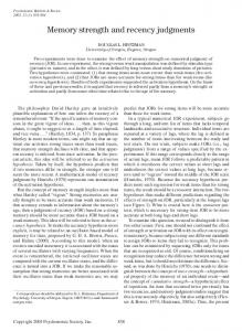
Figure 2. Predictions of rational models compared with the performance of participants from Lober and Shanks (2000, Experiments 4-6). Numbers along the top of the figure show stimulus contingencies.

2000). The term “graphical model” identifies a large class of formal models that have the common property of associating probability distributions with graphs. Several authors have proposed that graphical models provide a formal framework for dealing with questions about causality (eg. Pearl, 2000; Spirtes et al. 2000). Tutorials assuming different degrees of background knowledge are provided by Charniak (1991), Cowell (1998) and Heckerman (1998). The classic reference on the subject in artificial intelligence is Pearl (1988). Graphical models provide an intuitive representation for the dependency structure of probability distributions, expressing a distribution in terms of a graph in which the nodes are random variables, and edges between nodes indicate dependence. One of the most commonly used graphical models is a Bayesian network, in which the graph is directed and acyclic. Directed graphs are typically drawn with arrows indicating the direction of an edge, with “parent” nodes having arrows to their “children”. Recent work has used Bayesian networks to represent causal relationships, taking these directed edges as indicating a causal connection between parent and child (Pearl, 2000; Glymour, 1998; Glymour & Cooper, 1999; Spirtes et al. 2000). Here the causal structure is fundamental, with the probability distribution over the values of a variable a direct function of the values of its parents. The nature of the relationship between a variable and its parents is specified by the conditional probability distribution associated with that variable. For example, consider the directed graph denoted Graph1 in Figure 3, which we will later use in our development of a theory of elemen-

6

THOMAS L. GRIFFITHS

B

C

Graph 1

B

Parameter estimation and structure learning

C

Graph 0 E

E

Figure 3. Directed graphs involving three variables, B,C, E, relevant to elemental causal induction. B represents background variables, C a potential causal variable, and E the effect of interest. Graph1 , shown in (a), is assumed in existing rational accounts of causal induction. Computing causal support involves comparing the structure of Graph1 to that of Graph0 , shown in (b), in which C and E are independent.

tal causal induction. The effect node E is the child of two binary-valued parent nodes: C, the putative cause, and B, a constant background. The probability distribution P(E, B,C) can be specified by identifying P(B), P(C), and the conditional probability P(E|B,C). The conditional probability distribution associated with a node can be any probabilistically sound function of its parents. A range of such functions have been explored for continuous-valued variables, including some which explicitly relate Bayesian networks to artificial neural networks (e.g., Neal, 1992). Here, we consider two simple parameterizations for discrete-valued variables: linear and noisy-OR. A linear parameterization of Graph1 assumes that the probability of E occuring is a linear function of C. The result is Q(e+ |b, c; wB , wC ) = wB · b + wC · c,

(3)

where Q(·) is the probability distribution implied by the model (distinguished from P(·), the observed distribution), wB , wC are parameters associated with the strength of B,C respectively, and b+ = c+ = 1, b− = c− = 0 for the purpose of arithmetic operations. Because we are attempting to produce probabilities, we would need to constrain wB + wC to lie between 0 and 1, and these parameters reflect the relative strength of influence of B,C on E. Another parameterization we could use is the noisy-OR gate (Pearl, 1988). Just like the linear parameterization discussed above, this assumes that E can result from the presence of either B or C. The major difference is that this relationship is not strictly additive. Instead, a probabilistic relationship is assumed, in which the probability of e+ given b+ and c+ is computed as if B and C each had an opportunity to produce e+ independently: Q(e+ |b, c; wB , wC ) = 1 − (1 − wB )b (1 − wC )c .

(4)

This expression gives wB for the probability of e+ in the presence of b+ alone, and wB + wC − wB wC for the probability of e+ in the presence of both b+ and c+ . Both wB and wC are constrained to lie in the range [0, 1].

There are two kinds of learning involved in constructing a Bayesian network from a set of observed data: parameter estimation, by which the parameters associated with the conditional probabilities are identified, and structure learning, where the graphical structure expressing the causal structure of the variables is learned (Heckerman, 1998). In his discussion of psychological theories of causal induction, Glymour (1998) points out the importance of considering both of these aspects of learning in understanding causal induction. Here we examine how the notions of parameter estimation and structure learning can provide insight into modeling human causal judgments. Given a particular graphical structure and a parameterization, the Bayesian network that best accounts for a set of data can be found by estimating the parameters that, through the parameterization of the network, determine the conditional probability distributions. This process of parameter estimation is one of the basic steps in learning a Bayesian network from a set of observed data. There are several approaches to parameter estimation in Bayesian networks (Heckerman, 1998). The simplest approach is maximum likelihood estimation: taking the set of parameters that maximizes the probability of the data under the assumed graph structure. Both ∆P and causal power are maximum likelihood estimates of the causal strength parameter wC in Graph1 , but under different parameterizations (Tenenbaum & Griffiths, 2001). As shown in the Appendix, ∆P corresponds to the linear parameterization, whereas causal power corresponds to the noisyOR parameterization.3 ∆P and causal power are both maximum likelihood estimates of the parameters of a fixed graphical structure: they both measure the strength of a causal relationship, based upon the assumption that the relationship exists. By identifying both ∆P and causal power as maximum likelihood parameter estimates, we do not intend to minimize the important differences between them. In fact, this analysis helps to illustrate how these measures differ: they make different assumptions about the parameterization of a causal relationship. The linear relationship assumed by ∆P seems less consistent with the intuitions people express about causality than the noisy-OR, an important insight which is embodied in Cheng’s (1997) Power PC theory. The appropriate parameterization for the relationship between a cause and its effects will depend upon an individual’s beliefs about the “causal mechanism” by which those effects are brought about (cf. Ahn & Bailenson, 1996). For some causal mechanisms, the linear parameterization may be appropriate, for others, the noisy-OR. We can also specify parameterizations for effects that are not binary-valued, extending the idea of causal strength to more varied ways in which a cause might produce an effect. We will return to this possibility in Experiment 3. Both ∆P and causal power are estimates of the strength of a causal relationship, performing parameter estimation 3 Glymour (1998) first pointed out the connection between the Power PC theory and noisy-OR gates, but did not show that causal power is a maximum likelihood parameter estimate.

STRUCTURE AND STRENGTH IN CAUSAL JUDGMENTS

within a fixed causal structure. The central claim of this paper is that understanding the rational basis of human causal judgments requires considering the problem of learning causal structure. In terms of the graphical models in Figure 3, ∆P and causal power are concerned with the parameters of Graph1 . In contrast, we believe that human causal induction may be focused on trying to distinguish between Graph1 , in which C is a parent of E, and the “null hypothesis” of Graph0 , in which C is not. This binary decision is a result of the deterministic nature of the existence of causal relationships – either a relationship exists or it does not – a property of causality that is not captured by considering only the strength of a causal relationship (Goldvarg & JohnsonLaird, 2001). The structual inference as to whether the data were generated by Graph0 or Graph1 can be formalized as a Bayesian decision. Making this decision requires evaluating the evidence the data provide for a direct causal relationship between C and E – determining the extent to which those data are better accounted for by Graph1 than Graph0 . We will assume that Graph0 and Graph1 are parameterized as noisy-OR gates over one and two variables respectively. Having specified two clear hypotheses about the source of a set of data X, we can then compute the probabilities P(Graph0 |X) and P(Graph1 |X) by applying Bayes’ rule. The posterior probability of Graph1 indicates the extent to which an individual should believe in the existence of a causal relationship, but it may be more appropriate to model human judgments using a directly comparative measure, such as the log posterior odds (cf. Anderson, 1990; Shiffrin & Steyvers, 1997). In log odds form, we can write Bayes’ rule as log

P(X|Graph1 ) P(Graph1 ) P(Graph1 |X) = log + log (5) P(Graph0 |X) P(X|Graph0 ) P(Graph0 )

where the left hand side of the equation is the log posterior odds, and the first and second terms on the right hand side are the log likelihood ratio and the log prior odds respectively. Bayes’ rule stipulates how a learner should update his or her beliefs given new evidence, with the log posterior odds combining prior beliefs with the implications of the evidence. The effect of a set of observations X on the belief in the existence of a causal relationship is completely determined by the value of the log likelihood ratio. The log likelihood ratio is thus commonly used as a measure of the evidence a set of data provides for a hypothesis, and is also known as a Bayes factor (Good, 1961, Kass & Rafferty, 1995). We will use this measure to define “causal support”, the evidence a data set X provides in favor of Graph1 over Graph0 : P(X|Graph1 ) support(X) = log . (6) P(X|Graph0 ) To evaluate causal support, it is necessary to compute P(X|Graph1 ) and P(X|Graph0 ). These probabilities are defined in terms of just the underlying causal structure, and are obtained by summing over all values of the strength parameters. Graph0 uses a single parameter, wB , to describe the probability of the effect, this probability having the same

7

value regardless of whether the cause is present or absent. Graph1 has a second parameter, wC , that captures the effect of C on the probability of E. Since we are using a noisyOR parameterization, this second parameter corresponds to the quantity estimated by causal power. Causal support will covary with the estimated strength of a causal relationship, since strong relationships can be expressed much better in the two-parameter model. However, it will also be sensitive to what a frequentist statistician would refer to as the variance in the estimate of the strength of a causal relationship, which relates to the breadth of the posterior distribution over wC . The simple hypothesis of Graph0 will be preferred over the more complex Graph1 unless the posterior distribution over wC places most of its mass away from zero. Causal support is a measure of the evidence a set of observations provide for the existence of a causal relationship. It is thus one component of a rational account of causal induction, indicating the extent to which the data should lead us to change our beliefs. The other component is our prior beliefs, with the revised estimate of the probability of the data having been generated from Graph1 reflecting both priors and causal support. Just as ∆P and causal power provide measures of the strength of a causal relationship independent of domain, causal support does not take into account these prior probabilities. In general, we expect causal support to correlate with people’s judgments about causal relationships, but we anticipate that these judgments will also be influenced by priors. The details of evaluating causal support are given in the Appendix, where we also show that it can be approximated by Pearson’s χ2 test for independence. This approximation is best when the contingency table contains a large number of observations, and the potential cause has only a weak effect. Since χ2 is much simpler to compute than causal support, it provides a useful complement to causal support in modeling human judgments. The use of χ2 as a model of human causal induction has been considered by other authors, and rejected on the grounds that it does not reflect the asymmetry inherent in a causal relationship (Allan, 1980; Shanks, 1995b; Lopez et al., 1998). We also believe that χ2 should be treated with caution as a model of causal induction, because it only approximates causal support for large N. While χ2 is symmetric, causal support specifically postulates an asymmetric relationship between cause and effect, and produces different results when the roles of cause and effect are exchanged. While both χ2 and causal support address the structural question of whether a causal relationship exists, causal support uniquely postulates a specific form and direction for this causal relationship, which can sometimes lead to quite different predictions.

Empirical predictions of causal support Identifying the distinction between structure and strength in causal induction raises the question of when we should expect human judgments to reflect these different factors – a question we address in detail in the General Discussion. For now, we consider one of the data sets we discussed earlier

8

THOMAS L. GRIFFITHS

P(e+|c+) P(e+|c−) 100

0.90 0.80 0.70 1.00 1.00 1.00 1.00 1.00 0.80 0.40 0.90 0.66 0.33 0.00 0.75 0.50 0.25 0.00 0.60 0.40 0.00 0.83

Humans 50

0

Support

χ2

Figure 4. Predictions of structure-based rational models compared with the performance of human participants from Lober and Shanks (2000, Experiments 4-6). Numbers along the top of the figure show stimulus contingencies.

in which it was apparent that neither of the strength-based rational models could account for the data, suggesting some other factor may be involved. Figure 2 shows the data from Lober and Shanks (2000, Experiments 4-6). These experiments were conducted with the aim of producing results that could be predicted by the PCM but not the Power PC theory, and consequently the r2 values of 0.959 and 0.356 for ∆P and causal power respectively come as little surprise. However, it is noteworthy that the predictions of causal support and the χ2 approximation both give r2 values of 0.986, γ = 0.57, 0.5, which exceeds the result given by ∆P. One reason for the success of these structure-based models is that they are capable of capturing the non-monotonic relationship that neither the PCM nor the Power PC theory could predict. Both causal support and χ2 display a nonmonotonic relationship for these contingencies because the evidence for a causal relationship covary with both the estimated strength of a relationship and the variance of the estimate. In the case of causal support, this is because the evidence for a causal relationship is intimately dependent upon the posterior distribution over wC , the strength of the relationship: if the data suggest that wC is greater than zero, then causal support should be large. Whether or not wC is convincingly greater than zero will reflect both the apparent magnitude of wC , as might be estimated by causal power, and how much we believe this is the true magnitude, corresponding to the variance of the estimate. This formulation allows us to give an intuitive explanation for the non-monotonic relationship seen in the data. Assume

that the frequencies contributing to P(e+ |c+ ), P(e+ |c− ) are actually drawn from the same distribution, where E occurs with some probability p regardless of the value of C. This is the assumption of independence tested by both causal support and χ2 . Then the variance of the resulting frequencies will be proportional to p(1 − p). This variance is maximized when p = 0.5. If P(e+ |c+ ) and P(e+ |c− ) are both near 0.5 the difference between them – corresponding to the strength of the relationship – will have weaker implications than if one of them lies near 1 or 0. The structural measures of causal support and χ2 are sensitive to both the strength of a causal relationship and its variance. The PCM and the Power PC theory compute only the strength of the causal relationship, and cannot predict this kind of non-monotonicity. The non-monotonic pattern of responses suggests that people may be sensitive to both the apparent strength of causal relationships and how strongly we believe this is the actual strength, and is consistent with the predictions of causal support. These non-monotonicities cannot be accounted for by either the PCM or the Power PC theory. However, this response pattern was only observed in a single experiment conducted by Lober and Shanks (2000). In the remainder of the paper, we present a series of experiments that explore this effect, as well as further predictions of causal support. Experiment 1 examines whether the non-monotonic pattern of responses observed by Lober and Shanks can be replicated, over a range of values of ∆P and question types. Experiment 2 uses this effect to illustrate that asking questions that focus on structure and strength can dissociate these two aspects of causal learning in people’s responses. Experiment 3 uses the generality of explaining causal induction as a structural inference to predict people’s judgments in a situation where causes alter the rates at which their effects occur. All of these experiments will use the summary format, directly presenting participants with information about the frequency of events. We will motivate this choice in the General Discussion, where we turn to the question of when we expect judgments to be affected by structure and strength.

Experiment 1 Method Participants. A total of 321 undergraduates from Stanford University participated in the study for course credit. Participants were assigned to conditions at random, giving a total of 101 participants in the Cause condition, 125 in the Confidence condition, and 95 in the Strength condition. Materials. The experiment was conducted in survey form, featuring detailed instructions about the task and then obtaining ratings on a total of 14 different contingency structures. The instructions placed the problem of causal induction in a medical context, reading: Imagine that you are working in a laboratory and you want to find out whether certain chemicals

9

STRUCTURE AND STRENGTH IN CAUSAL JUDGMENTS

cause certain genes to be expressed in mice. Below, you can see laboratory records for a number of studies. In each study, a sample of mice were injected with a certain chemical and later examined to see if they expressed a particular gene. Each study investigated the effects of a different chemical on a different gene, so the results from different studies bear no relation to each other. Of course, these genes may sometimes be expressed in animals not injected with a chemical substance. Thus, a sample of mice who were not injected with any chemical were also checked to see if they expressed the same genes as the injected mice. Also, some chemicals may have a large effect on gene expression, some may have a small effect, and others, no effect. Contingencies described how many mice from a sample of 100 expressed a particular gene. For example, for one chemical and one gene, participants would be informed that 2 out of 100 injected mice expressed the gene, and 0 out of 100 uninjected mice expressed the gene. The exact instructions on how to rate the strength of the causal relationship differed across three conditions, to establish that the results were not due to the use of a specific wording in the question. Participants in the Cause condition were given instructions designed to elicit a direct judgment about the nature of the causal relationship between the two variables: For each study, write down a number between 0 and 20, where 0 indicates that the chemical DOES NOT CAUSE the gene to be expressed at all, and 20 indicates that the chemical DOES CAUSE the gene to be expressed every time. Participants in the Confidence condition received instructions that were intended to produce responses more indicative of the subjective probability that a relationship existed: For each study, write a number between 0 and 20, where 0 indicates COMPLETE CONFIDENCE that the chemical DOES NOT HAVE AN EFFECT on whether the gene is expressed and 20 indicates COMPLETE CONFIDENCE that the chemical DOES HAVE AN EFFECT on the gene’s expression. Use intermediate ratings to indicate degrees of belief between these extremes; use 10 – the middle value – to indicate NO CONFIDENCE at all about whether or not the chemical has any effect. Finally participants in the Strength condition were asked to directly assess the strength of the causal relationship: For each study, write down a number between 0 and 20, where 0 indicates that the chemical has the WEAKEST POSSIBLE effect on whether the gene is expressed and 20 indicates that the chemical has the STRONGEST POSSIBLE effect on whether the gene is expressed.

P(e+|c+) P(e+|c−)

100 60

70 30

40 / 100 0 / 100

100 93

53 46

7 / 100 0 / 100

100 98

51 49

2 / 100 0 / 100

20 15

Cause

10 5 0 20 15

Confidence

10 5 0 20 15

Strength

10 5 0

Figure 5. Performance of human participants in Experiment 1. Each graph shows responses for different sets of contingencies in one instruction condition. The numbers across the top of the figure show the relevant contingencies. The pattern of responses was not strongly affected by the instructions, and in each case nonmonotonic judgments consistent with the predictions of causal support were observed. Error bars indicate one standard error.

Participants in all conditions then saw the same set of contingencies, with order randomized across individuals. The contingencies were selected to give three different groups in which non-linearities could occur. In addition to these nine pairs of contingencies, there were five distractor pairs. The critical sets were {0.40, 0.00}, {0.70, 0.30}, {1.00, 0.60}, for which ∆P = 0.40, {0.07, 0.00}, {0.53, 0.46}, {1.00, 0.93}, for which ∆P = 0.07, and {0.02, 0.00}, {0.51, 0.49}, {1.00, 0.98}, for which ∆P = 0.02.

Results and Discussion The means for the three critical sets of contingencies are shown in Figure 5, broken down by condition. A two-way within-between ANOVA showed a main effect of condition, F(2, 318) = 16.90, MSE = 74.10, p < 0.001, but no interaction between condition and the effect of the different contingencies on response, F(16, 2544) = 0.97, MSE = 17.13, p = 0.48. Given the large number of participants in the experiment, the inability to reject the null hypothesis of no interaction suggests that question type has a negligible effect on the pattern of responses we observed. For each set of contingencies and each condition, we tested for the presence of a quadratic trend. This test is sensitive to non-linear patterns of responding, which are only predicted by causal support and, to a lesser degree, causal power. As can be seen from the figure, in each case where we found a significant non-linear trend the pattern of means was actually

10

THOMAS L. GRIFFITHS

non-monotonic, a result that can be predicted only by causal support. All comparisons had degrees of freedom (1, 2552) and MSE = 17.13. Significant quadratic trends were found for ∆P = 0.40 in all groups, F = 10.53, 7.92, 9.40 for Cause, Confidence, and Strength respectively, all p < 0.005, and likewise for ∆P = 0.07 (F = 10.85, 10.95, 10.75 respectively, p < 0.005 for each. The quadratic trends were marginally significant for ∆P = 0.02, F = 2.91, 2.78, 2.24 respectively, with p = 0.088, 0.096, 0.13. To ensure that the non-monotonicities we found were also observable at the level of individual participants, we examined the proportion of subjects producing non-monotonic response patterns. Of the 101 participants in the Cause condition, 27, 33, and 19 showed the predicted non-monotonic response for the critical sets with ∆P = 0.40, 0.07 and 0.02 respectively, and 57 participants, over half the sample, produced a non-monotonic response at least once. For the sake of comparison, we also examined how many instances of the response pattern predicted by causal power and ∆P were evident in the sample: 19, 11, and 7 gave responses in an order consistent with causal power, and 6, 9, and 36 gave the same answer for all three contingencies, as predicted by ∆P. Similar results were observed in the other two conditions. Of the 125 participants in the Confidence condition, 34, 37, and 24 produced non-monotonic responses for the three sets of contingencies, with 70 participants showing the non-monotonic response pattern at least once. Only 13, 14, and 13 participants showed responses consistent with causal power, and 13, 15 and 31 gave identical answers for all three contingencies. In the Strength condition, 35, 27 and 12 of the 95 participants showed non-monotonic response patterns for the critical sets, and 55 did so at least once. 1, 8, and 7 participants showed responses consistent with causal power, while 15, 12, and 29 produced the pattern predicted by ∆P. To obtain a quantitative measure of the correspondence of the data with the different models, we correlated the predictions of each model with the mean of the responses across all three conditions. Causal support and χ2 gave r2 = 0.933 and 0.974 respectively, with γ = 0.68, 0.54. ∆P achieves a correlation comparable to support and χ2 with r2 = 0.970, γ = 0.47 because the non-monotonicities contribute only weakly to the total variance. Causal power gives a poor fit to the data, with the best results obtained as γ approaches zero. Causal power predicts strong trends that are inconsistent with the data, and these trends are minimized by the power transformation for small values of γ. With γ < 0.01, causal power gives r2 ≈ 0.25. The plotted values for causal power use γ = 0.01. The results support the predicted non-monotonic effect: in a set of contingencies with the same ∆P, the situations involving more extreme probabilities show increased judgments of the strength of the causal relationship. Nonmonotonic patterns of responses similar to those observed by Lober and Shanks (2000) were replicated in three different instruction conditions, suggesting that the effect is not a consequence of a particular set of instructions. PCM and the Power PC theory predict that ratings should either decrease monotonically or remain constant. Thus, while ∆P gives a

P(e+|c+) 100 P(e+|c−) 60

70 30

40 / 100 0 / 100

100 93

53 46

7 / 100 0 / 100

100 98

51 49

2 / 100 0 / 100

20 15 10

Humans

5 0

∆P

Power

Support

χ2

Figure 6. Predictions of computational models for contingencies used in Experiment 1. The first panel shows the mean of the human data across all three conditions. Numbers along the top of the figure show stimulus contingencies.

good quantitative account of the data, both models are qualitatively inconsistent with the results.

Dissociating structure learning and parameter estimation Experiment 1 provides evidence that people’s predictions are consistent with causal support, demonstrating a sensitivity to both the estimated strength of a relationship and the variance of this estimate. This sensitivity suggests that the judgments people make in causal induction tasks may be a consequence of evaluating a structural question about whether or not a causal relationship exists. However, structure learning forms only part of causal induction. Once the causal structure of a situation is known, it becomes appro-

11

STRUCTURE AND STRENGTH IN CAUSAL JUDGMENTS

priate to ask questions about the strength of causal relationships within that structure. Under different circumstances, we might expect causal judgments to reflect aspects of both structure learning and parameter estimation. For problems where the relationship between causes and effects is like that of the noisy-OR, causal support is a structural measure while causal power estimates the strength of a causal relationship. These two quantities express different aspects of causal induction, and should be dissociable. In particular, judgments that are explicitly structural should correspond more closely to causal support, and judgments that explicitly assume a causal structure should correspond more closely to causal power. One kind of judgment that requires the assumption of a causal structure is assessing a counterfactual statement. Pearl (2000) presents a formal theory of counterfactuals, providing a method for obtaining answers to questions like “What is the probability that a mouse not expressing the gene before being injected will express it after being injected with the chemical?”. Pearl’s theory involves a simple procedure for evaluating such queries using causal Bayesian networks, which assumes a specific network structure and then performs probabilistic computations that explicitly reflect the parameters of the network. In the case of the network shown in Figure 3 (a), the answer to the counterfactual question given above corresponds exactly to the quantity that Cheng (1997) calls causal power. Several researchers have recently begun to use counterfactual questions as a means of eliciting causal judgments consistent with the Power PC theory. Collins and Shanks (in press) showed that asking a counterfactual question produces results more consistent with causal power in an online causal induction task. Buehner et al. (submitted) use a procedure in which participants are first asked to judge whether a causal relationship exists, and then give counterfactual responses in those cases where they believe that this is the case. Based upon the relationship between counterfactual queries and model parameters, the initial judgment about whether one variable has an effect on another should not be necessary in order to elicit responses that reflect strength parameters. However, this initial judgment is explicitly a structural judgment: it requires a binary decision about whether a relationship between two variables exists, which is a structural question. Hence, this paradigm may provide a means of finding the expected dissociation between structural and parametric aspects of causal induction. The aim of Experiment 2 was to try to dissociate structural and parametric aspects of causal induction by asking different kinds of questions. Based upon the relationship between counterfactual queries and strength parameters, we expected that asking a counterfactual question would elicit responses more consistent with causal power. We also predicted that responses to questions requiring binary judgments about whether one variable has an effect on another would more strongly reflect structural considerations, and thus be closer to causal support and its χ2 approximation.

Experiment 2 Method Participants. A total of 234 undergraduates from Stanford University participated in the experiment for course credit. Each participant was randomly assigned to one of four conditions, detailed below, with 66 (Causal, Rating only), 60 (Causal, Effect and Rating), 47 (Counterfactual, Rating only), and 61 (Counterfactual, Effect and Rating) participants per group. Materials. As in Experiment 1, materials consisted of a short survey describing the task and eliciting judgments on 11 pairs of contingencies providing frequency information corresponding to the entries a, b, c, d in Table 1. These contingencies corresponded to those used in Experiment 1, omitting three of the distractors. Ratings were elicited on a scale from 0-100, since some of the questions explicitly concerned probabilities. In order to confound trivial response strategies, the total frequencies were set to be 60, rather than 100. Thus participants would receive information that 2 out of 60 injected mice expressed the gene, while 0 out of 60 uninjected mice expressed the gene. The values of ∆P held constant across the different stimuli were also changed slightly, becoming 0.40, 0.12, and 0.03, but the survey otherwise followed the format of that used in Experiment 1. The specific questions asked of the participants are detailed below. Procedure. Participants were split into four conditions, in a 2 × 2 between-subjects factorial design. The factors were the kind of question that participants were asked (Causal or Counterfactual), and whether they had to decide whether there was an effect of the chemical on the gene prior to answering this question. The causal question involved directly assessing the causal relationship between C and E, and the counterfactual question asked for the probability that introducing C will produce E, in a case where E has not occurred. The instructions for the causal question corresponded to those used in the Cause condition of Experiment 1: For each study, write down a number between 0 and 100 representing the probability that the chemical causes the gene to be expressed. A probability of 0 indicates that the chemical DOES NOT CAUSE the gene to be expressed at all, and a rating of 100 indicates that the chemical DOES CAUSE the gene to be expressed every time. Use intermediate ratings to indicate degrees of causation between these extremes. In contrast, the instructions for the counterfactual question read: For each study, write down a number between 0 and 100 representing the probability that a mouse not expressing the gene before being injected will express it after being injected with

12

THOMAS L. GRIFFITHS

the chemical. A probability of 0 indicates COMPLETE CONFIDENCE that the mouse WILL NOT EXPRESS THE GENE, and a probability of 100 indicates COMPLETE CONFIDENCE that the mouse WILL EXPRESS THE GENE. Use intermediate ratings to indicate degrees of confidence between these extremes. For each of these questions, one group of participants simply answered the question (Rating only), while another group first made a yes/no judgment about whether the chemical affects gene expression (Effect and Rating). This latter group only answered the causal or counterfactual question in the cases where they believed that there actually was an effect.

P(e+|c+)

60

42

24 / 60

60

33

7 / 60

60

31

2 / 60

P(e+|c−)

36

18

0 / 60

53

26

0 / 60

58

29

0 / 60

100

Causal question only

50

0 100

Counterfactual question only

50

0

Results and Discussion The results are shown in Figure 7. The effect judgments were collapsed across the causal and counterfactual questions, since they represented an assessment of the nature of the causal relationship that was made prior to and independently from the kind of question that was being asked. The responses to the causal and counterfactual questions and the effect judgments were all analyzed separately. In each case, the effect of the baseline probability P(e+ |c− ) was assessed for each of the groups of stimuli with the same value of ∆P. The responses to the causal question alone showed the predicted non-monotonicities. Quadratic trend analyses within each of the critical sets of contingencies gave statistically significant results in the first two cases, F = 7.59, 4.80, p < 0.05 for both, and a marginally significant result for the third, F = 3.41, p = 0.065. Weak linear trends were shown in all three sets of contingencies, F = 8.70, 5.83, 3.92, p < 0.05 in each case. All comparisons had degrees of freedom (1, 650) and MSE = 401.68. Of the 66 participants, 19, 20, and 12 showed the non-monotonic response pattern on the critical sets of contingencies. By comparison, 18, 8, and 7 participants showed the pattern consistent with causal power, and 7, 8, and 20 showed the pattern consistent with ∆P. These results replicate those in the Cause condition of Experiment 1, demonstrating the predicted non-monotonicities in the first two groups. A different pattern was shown for the responses to the counterfactual question alone, where none of the quadratic trends were statistically significant, F = 2.63, 1.36, 2.01, p = 0.11, 0.24, 0.16 respectively. Instead, we found strong linear trends in each set, F = 15.87, 47.68, 47.38, p < 0.0001 for all three cases. All comparisons had degrees of freedom (1, 460) and MSE = 559.83. These linear trends are consistent with causal power, as might be expected from asking this counterfactual question. Of the 47 participants, 17, 7, and 12 responded in a way consistent with causal support, while 16, 21 and 16 showed the response pattern consistent with causal power and 1, 4, and 5 showed the pattern predicted by ∆P. The yes/no effect judgments showed no linear trends, and strong non-monotonicities, as we would expect for a purely structural judgment. The first set of contingencies suffered from a strong ceiling effect, and showed no significant trends, F = 0.59, 0.05, p = 0.44, 0.82 for linear and quadratic trends

1

Effect judgment (Y/N)

0.5

0 100

Causal with Effect judgment

50

0 100

Counterfactual with Effect judgment

50

0

Figure 7. Results of Experiment 2. The first two graphs show responses in the Causal and Counterfactual conditions when only ratings were given by the participants. The third graph shows the probability that a participant would believe there was a causal relationship, for each set of contingencies. These effect judgments were collapsed across Causal and Counterfactual questions. The final two graphs show the ratings given after effect judgments were made, restricted to those participants who believed that there was a relationship. Error bars indicate one standard error.

respectively. In the other two sets of contingencies, linear trend analyses gave F = 3.34, 0.15, p = 0.07, 0.70, while quadratic analyses gave F = 34.05, 14.27, p < 0.001 for both tests. All comparisons had degrees of freedom (1, 1200) and MSE = 0.11. The non-monotonicities shown in the second and third sets of contingencies were much more pronounced than those seen for the other questions. Unfortunately, analyzing these data for individual subject response patterns was complicated by the fact that the responses were binary, with many responses being either 111 or 000. Of the 5 participants who did not give the same response to all three contingencies

STRUCTURE AND STRENGTH IN CAUSAL JUDGMENTS

in the first set, 1 showed the predicted pattern. Of the 56 and 29 giving distinct responses to the second and third sets, 24 and 9 showed the non-monotonic pattern respectively. No subjects showed the response pattern consistent with causal power. Analysis of the responses to the causal and counterfactual questions following the effect judgment raises the question of how to score cases where participants judged there to be no effect. Assigning a value of zero to these cases and averaging them together with the other judgments would result in an implicit influence of the initial effect upon the analysis of the responses to the causal and counterfactual questions, confounding the influences of structure and strength on the responses. In the current context, the fact that the effect judgments remain the same across these conditions also means that assigning values to the cases where no relationship was judged to exist artificially brings the judgments closer together. In light of this issue, we present the responses only in those cases where participants judged a relationship to exist. As can be seen from Figure 7, the resulting responses resemble those made without a prior effect judgment, except in the group where ∆P is low. In this group, the omission of low scores as a consequence of negative effect judgments inflates responses to both questions, and the large standard errors indicate the low reliability of these estimates. Consequently, we do not discuss these data further. The predictions of causal power and causal support, together with the χ2 approximation, were fit to the responses to the causal and counterfactual questions, and the effect judgments. Since the contingencies used in this experiment were close to those of Experiment 1, the predictions of the models resemble those shown in Figure 6. For the causal question, causal power gives a fit of r2 = 0.368, with γ = 0.01, while causal support and χ2 give r2 = 0.955, 0.957 respectively, with γ = 0.80, 0.75. In contrast, the counterfactual question gives a fit of r2 = 0.759 for causal power, with γ = 0.07, and r2 = 0.776, 0.637 for support and χ2 respectively, with γ = 0.59, 0.73. Asking the counterfactual question considerably increases the fit of causal power to the responses, and decreases the fit of causal support and the χ2 approximation. The counterfactual question thus increased the correspondence of the results with causal power, an outcome which extends the results of Collins and Shanks (in press) to a task with a summary format and a range of contingencies. For the effect judgments, causal power again gives a low r2 = 0.309, with γ = 0.01, while both causal support and χ2 give higher r2 = 0.821, 0.912 respectively, with γ = 0.50, 0.40. These results are consistent with our predictions: the causal question appears to represent some combination of structural and parametric considerations, while these can be more directly tapped by asking different kinds of questions. Asking counterfactual questions produces results more consistent with causal power, which is a parameter estimate. Asking for direct binary decisions about whether one variable affects another produces stronger non-monotonicities, reflecting greater sensitivity to structural factors. The results of this experiment suggest that structure learning and parameter estimation are dissociable aspects of

13

causal induction. These two kinds of learning are applicable in different contexts – structure learning, as represented by causal support, is appropriate in contexts where the central question is whether a causal relationship exists. Parameter estimation, as represented by ∆P and causal power, assumes that the causal relationship exists, and gives a measure of its strength. This strength will influence the probability of the effect in the presence of the cause, and thus allows the assessment of counterfactual queries. The distinction between these two kinds of questions about causal relationships helps to indicate the contexts in which one kind of learning might be expected to predominate. In the General Discussion we will consider other factors that might influence whether a judgment draws upon structure or strength.

Causal induction with rates Experiments 1 and 2 provide evidence for the importance of structural considerations in causal induction, as measured by causal support and the χ2 approximation. The expression for causal support has a close correspondence to a model of causal induction proposed by Anderson (1990; Anderson & Sheu, 1995). Anderson’s theory was not motivated by graphical models, but employed the same solution of assessing the posterior odds in favour of a situation in which C and E were not independent. Beyond the connection to graphical models, the main differences between the present account and Anderson’s theory are the choice of probability distributions and the treatment of parameters. In Anderson (1990), distributions are established through the selection of at least four model parameters that are optimised for each data set. In contrast, the present model incorporates no free numerical parameters, integrating over the terms in the likelihood. The present work represents an advance over that of Anderson (1990; Anderson & Sheu, 1995) in two respects. Firstly, Anderson exhibited no data that provided evidence in favor of his theory. Anderson (1990) considered only existing data sets, and found no empirical phenomena that his model explained that could not be accounted for by an appeal to ∆P. Similar results were obtained by Anderson and Sheu (1995, Experiment 1), who found that a version of ∆P with the same number of free parameters as their Bayesian model gave a better fit to the data. Our experiments demonstrate an effect that is not consistent with either ∆P or causal power, and that can be explained without needing additional parameters. Secondly, the use of graphical models in specifying causal support gives our approach a great deal of generality. While we have focused so far on inferring the existence of a single causal relationship from contingency data, causal support is defined for the comparison of two graphical structures under any parameterization. Thus, the observations from which the existence of causal relationships can be established need not be contingencies. This generality also extends to the other theories that we have considered in this paper. The PCM and the Power PC theory suggest that causal induction is sensitive to the maximum likelihood estimate of the strength parameter describing the relationship between two variables un-

14

THOMAS L. GRIFFITHS

der different parameterizations. While the PCM and Power PC theory are concerned with causal induction from contingency data, this notion can be generalized to make predictions about different kinds of variables. In the remainder of the paper, we consider a case of causal learning that goes beyond contingency data, examining the roles of structure and strength in learning from the rates at which events occur. Anderson and Sheu (1995, Experiment 2) conducted an experiment in which participants learned whether clicking on a flute icon caused a change in the rate of musical notes produced by the flute. They found that judgments about the strength of the causal relationship were poorly predicted by the difference in rates for clicking and non-clicking intervals, an analogue of ∆P defined as ∆R = N(c+ ) − N(c− )

(7)

where N(c+ ) is the number of events in the interval when the cause, in this case clicking on the flute, was present, and N(c− ) is the number of events when the cause was absent. In fact, performance could be better predicted by “grating contrast”, which they defined as G=

N(c+ ) − N(c− ) N(c+ ) + N(c− )

(8)

and justified by its use in psychophysical research. Anderson and Sheu’s (1995) experiment used rate information rather than contingencies. Rate information, such as the number of events that occur in a time period, differs from contingency information in that the number of times the event did not occur is unknown. The outcome variable is thus of a different kind from that used to model contingency data, and requires a different parameterization for the underlying causal model. In particular, it requires a parameterization that can explicitly capture the rate at which events occur. The Poisson distribution provides a simple statistical model for the number of events that occur within a fixed interval. Using the Poisson distribution, the number of events occurring will have probability P(n) = e−λ

λn , n!

(9)

where λ is the Poisson rate parameter. This distribution can be derived by assuming that the amount of time between successive events follows an exponential distribution. We can use the Poisson distribution to define a parameterization for Graph0 and Graph1 that is an extension of the noisy-OR gate to continuous time. Under a noisy-OR parameterization where the event E has parents B and C, the probability of E if either B or C are present is wB or wC , and the probability of E with both present is wB + wC − wB wC , where the last term corrects for double-counting the cases in which both B and C would have produced E. Extending this model to the case where events are emitted over a continuous interval, the probability of an event at any point in time is simply the sum of the probabilities for each of the parents. Since the probability of two events from a Poisson process occurring simultaneously is zero, the resulting process is the sum of the

Poisson processes associated with the parents. The sum of two independent Poisson process is a Poisson process, with a rate determined by the sum of the rates of the original processes. This gives us the parameterization P(n|b, c; wB , wC ) = e−(bλB +cλC )

(bλB + cλC )n . n!

(10)

where λB is the rate associated with B, and λC is the rate associated with C. Using the parameterization given in Equation 10, we can define causal support as in Equation 6, where Graph0 is the model in which B is the only parent of E, and Graph1 is the model in which both B and C are parents of E. The details of the model are provided in the Appendix, where we also justify the approximation χ2 =

(N(c+ ) − N(c− ))2 . N(c− )

(11)

This approximation bears the same relationship to causal support for rates as the Pearson χ2 test for independence does for contingency data: it is a frequentist independence test that will be asymptotically equivalent to causal support. The role of the denominator in both χ2 and Anderson and Sheu’s (1995) grating contrast G may account for the success of the latter measure in explaining their results. Under the model specified by Equation 10, ∆R is the maximum likelihood parameter estimate for λC and is thus an appropriate measure of causal strength. The correspondence to ∆P and causal power can be seen by taking the rate information as just the positive events in a contingency table where the total sample size is unknown, so N(c+ ) = NP(e+ |c+ ) and N(c− ) = NP(e+ |c− ) for unknown N. If we assume that N is fixed across different experiments, we can obtain estimates consistent with the ordering and magnitude implied by ∆P using ∆R = N(c+ ) − N(c− ) = N∆P. If we make the further assumption that N is very large, ∆R will also correspond to causal power, since P(e− |c− ) will tend to 1. Performing causal induction with rate information goes beyond the standard contingency table format used in causal induction experiments, and requires the assumption of a different underlying statistical model. Having defined such a model, we can derive measures that reflect learning about causal structure and strength. The aim of Experiment 3 is to compare the predictions of these different measures with human performance on a causal induction task that involves rate information rather than contingencies.

Experiment 3 Method Participants. 82 Stanford University undergraduates took part in the study.

15

STRUCTURE AND STRENGTH IN CAUSAL JUDGMENTS

Materials. A short questionnaire outlined a hypothetical laboratory as follows:

N (c+) 100 N (c−) 50

60 10

52 2

60 50

20 10

12 2

52 50

12 10

4 2

100

Humans

Imagine that you are working in a laboratory and you want to find out whether electrical fields influence the radioactive decay of certain chemical compounds. Below, you can see laboratory records for a number of studies. In each study, a sample of some particular compound was placed inside a particular kind of electrical field for one minute, and the rate of radioactive decay was measured (in number of particles emitted per minute). Each study investigated the effects of a different kind of field on a different kind of chemical compound, so the results from different studies bear no relation to each other. Of course, the chemical compounds can emit particles even when not in an electrical field, and they do so at different rates. Some compounds naturally decay at a fast rate, while others naturally decay at a slow rate. Thus, the decay rate of each compound was also measured for one minute in the absence of any electrical field. For each study below, you can see how many particles were emitted during one minute inside the electrical field, and during one minute outside of the electrical field. What you must decide is whether the electrical field increases the rate of particle emissions for each chemical compound. The questionnaire gave a summary of nine experiments involving different chemical compounds and electrical fields, giving the number of particle emissions inside and outside the electrical field. The number of particle emissions in each example was selected to give three critical sets of rates: {52, 2}, {60, 10}, {100, 50}, for which ∆R = 50, {12, 2}, {20, 10}, {60, 50} for which ∆R = 10, and {4, 2}, {12, 10}, {52, 50}, for which ∆R = 2. There is no simple way to convert these counts into probabilities, other than assuming some hypothetical upper bound on the number of particle emissions. Procedure. Participants were given the questionnaire, and instructed to provide ratings in response to a question like that of the Cause condition in Experiment 2. Ratings were made on a scale from 0 (the field definitely does not cause the compound to decay) to 100 (the field definitely does cause the compound to decay).

Results and Discussion The results of the experiment are shown in Figure 8. We used linear and quadratic trend analyses to examine the results within each critical set of rates. All comparisons have degrees of freedom (1, 648) and MSE = 544.18. Both linear and quadratic trends were statistically significant in the first

50

0

∆R

Power (N = 150)

Support

2

χ

Figure 8. Results of Experiment 3. The top panel shows the responses given by the human participants to each of the nine sets of particle emission frequencies, which are shown along the top of the graph. Error bars indicate one standard error. The remaining figures show the predictions of computational models based on learning causal strength and structure. The results for causal power are based on a hypothetical maximum emission frequency N of 150, to illustrate that the trends are inconsistent with causal power even when artificially converted into probabilities. As N becomes large, causal power will come to resemble ∆R.

set, with F = 29.90, p < .0001 and F = 5.42, p < .05 respectively. Only the linear trend was significant in the second set, F = 69.86, p < 0.0001, with the quadratic trend giving F = 2.57, p = 0.11. The same pattern was observed for the third set, with F = 10.53, p < 0.005 for the linear trend and F = 0.98, p = 0.32 for the quadratic trend. Since ∆R predicts that responses within each of the critical sets should be constant, the significant linear and quadratic trends suggest that responses reflect the results of structural considerations. To examine this possibility, we evaluated the fit of ∆R, causal power, causal support, and

16

THOMAS L. GRIFFITHS

χ2 to the data. ∆R gave r2 = 0.807 with γ = 0.05. Causal power assumes the wrong statistical model for this kind of data, but might be applied if we assumed that participants were comparing the rates to some hypothetical maximum number of particles that might be emitted, N. As N approaches infinity, causal power converges to ∆R. The trends predicted by causal power do not vary with the choice of N, so the value N = 150 was chosen to allow these trends to be illustrated. The predicted trends are clearly at odds with those observed in the data, giving a fit of r2 = 0.714 with γ = 0.06. Causal support and χ2 gave better fits, with r2 = 0.957, γ = 0.35 and r2 = 0.962, γ = 0.01 respectively. The model predictions are shown in Figure 8, and demonstrate that a structural approach can account for the pattern of responses observed in the experiment. The success of causal support in this experiment provides further evidence for the primacy of structural considerations in causal induction. The goal of this experiment was to explore the roles of structure and strength in causal induction when the data indicating a causal relationship cannot be expressed in a contingency table. In a situation in which a causal relationship could be established by examining the rates of events in different contexts, people produced responses consistent with a structural inference. Holding the strength-based measure ∆R constant, we observed a pattern of responses that were consistent with the predictions of causal support and the χ2 approximation. This pattern of responses can be explained in terms of a structural inference about whether or not a causal relationship exists. Since rates of events are the basis for large amounts of both associative and causal learning, these results provide an illustration of the role that structural inferences might play in naturalistic cases of causal induction.

General Discussion Learning about causal structure is an important component of human causal induction. Using graphical models, we have shown that the two leading rational theories – the Probabilistic Contrast Model and the Power PC theory – both correspond to parameter estimation on a fixed graph. They do not consider the causal structure of a situation, instead assessing the strength of a causal relationship on the assumption that the causal relationship exists. The question of whether a particular causal relationship exists can be addressed as a Bayesian inference concerning graphical structures, and we term the evidence used in this inference “causal support”. For weak causal relationships described by a large amount of data, causal support can be approximated by the familiar χ2 statistic. Causal support accounts for aspects of the data that were not predicted by the PCM and the Power PC theory. In particular, these theories do not predict non-monotonicities in judgments about relationships resulting from extreme contingencies. Experiment 1 demonstrated that these nonmonotonicities arise in several sets of contingencies, and showed that neither the PCM nor the Power PC theory could account for these results. Experiment 2 showed that these

non-monotonicities can be removed by asking questions that assume a fixed causal structure, suggesting that it is possible to dissociate structure learning and parameter estimation in human judgments. Experiment 3 showed that similar trends provide evidence for structure learning in causal induction from rates, going beyond the contingency table format used in most studies of causal induction. The data presented in this paper suggest that structural factors play an important role in human causal induction. Considering causal structure as well as the strength of causal relationships provides the potential to produce more comprehensive rational models of causal judgments, and consequently to account for many of the phenomena of human performance that have previously been difficult to explain. In the following sections we discuss how particular tasks might influence the involvement of structure and strength in responses, consider how causal support relates to the notion of reliability introduced by Buehner and Cheng (1997), and outline the relationship between causal support and other work involving Bayesian networks in both psychology and computer science.

Factors affecting the importance of structure and strength The experiments presented in this paper suggest that people’s judgments about causality reflect two important properties of causal relationships: structure and strength. Experiment 2 showed that different kinds of questions about causal relationships produced responses that emphasized one of these aspects. This raises the question of what other factors might influence whether structure or strength will play a greater role in a particular judgment. When using classical statistics to analyse data from an experiment, psychologists are trained to first apply some form of significance test to establish whether an effect is present, and then to examine the size of that effect. We will suggest that a similar pattern might underlie human causal inference: our earliest judgments are about structure, since it may not be apparent whether a relationship really exists, while strength plays a greater role once this uncertainty is resolved. Experiments on causal induction are typically conducted either in an online format, where participants view separate trials in which a causal variable may or may not produce the effect, or via the presentation of summary data in the form of a contingency table. These different forms of presentation may have an impact on whether responses tend to reflect structure or strength. In particular, online tasks with a large number of presentations provide ample opportunity for structural questions to be resolved early in learning, meaning that later responses might be more likely to reflect the strength of the causal relationship. We would expect structural uncertainty to have a greater influence in the first few trials of online learning, or when presented data are presented in a summary format and only a single judgment is made. The experiments conducted in this paper all used the summary format, and showed evidence of being influenced by structural considerations. Strutural inferences also seem to

STRUCTURE AND STRENGTH IN CAUSAL JUDGMENTS P(e+|c+) 1.00 0.75 0.50 0.25 0.00 1.00 0.75 0.50 0.25 1.00 0.75 0.50 1.00 0.75 1.00 P(e+|c−) 1.00 0.75 0.50 0.25 0.00 0.75 0.50 0.25 0.00 0.50 0.25 0.00 0.25 0.00 0.00 100

Humans 50

0

Support

χ2

Figure 9. Predictions of structure-based rational models compared with the performance of human participants from Buehner and Cheng (1997, Experiment 1B). Numbers along the top of the figure show stimulus contingencies.

underlie early performance in online tasks. Experiment 1B of Buehner and Cheng (1997), presented in the introduction and in Figure 1 as a problem for both the PCM and the Power PC theory, was an online study with a total of 16 trials. In Figure 1, the data from Buehner and Cheng (1997, Experiment 1B) show that human judgments of the strength of the causal relationship between C and E vary systematically over contingencies where ∆P and causal power are constant. In addition, neither the PCM nor the Power PC theory predicts the increase in judgments as a function of P(e+ |c− ) when ∆P is zero. As stated above, ∆P and causal power gave r2 values of 0.791 and 0.776 respectively. The predictions of causal support and the χ2 approximation are shown in Figure 9. Causal support accounts for both of the trends that could not be predicted by ∆P and causal power, with an r2 value of 0.914, γ = 0.69. χ2 performs at the level of ∆P and causal power, with r2 = 0.790, γ = 0.60, but is inconsistent with a number of trends in the data. For these data, the number of observations contributing to the contingencies in each situation are sufficiently low that χ2 gives a poor approximation to causal support. The intuitive explanation for the predictions of causal support in the cases where ∆P = 0 is similar to the explanation given by Cheng (1997) for the need to include P(e+ |c− ) when computing causal power. When conducting experiments, psychologists are very sensitive to the possibility of producing null results through ceiling effects. When P(e+ |c− ) = 1.00, we have the ultimate ceiling effect: it is impossible to increase the probability of E occuring. To

17

a certain extent, this fact is reflected in the predictions of the Power PC theory, since causal power is undefined when P(e+ |c− ) = 1.00. However, neither the Power PC theory nor the PCM reflects the potential for ceiling effects in other cases where ∆P = 0. If P(e+ |c− ) = 0.75, there are far fewer cases that could potentially be affected by a causal relationship between C and E. Not only should ∆P have a greater influence on judgments in this context, as stated in causal power, but the fact that ∆P = 0 should be given less weight. Any relationship between C and E that is expressed in this context will be taken to be stronger, and correspondingly the lack of an effect can be consistent with a stronger relationship between C and E. The causal support model is sensitive to this fact, leading to predictions consistent with human performance on these contingencies. Experiments using longer online tasks also provide support for the hypothesis that structure affects early judgments, and strength later judgments. Shanks and colleagues have conducted a number of studies in which causal strength seems to dominate after many online trials (Lober & Shanks, 2000; Perales & Shanks, in press; Shanks, 2002). One particularly relevant result comes from Lober and Shanks (2000), where the non-monotonic pattern of responses that motivated our Experiment 1 was not apparent when the same contingency data were presented online (Lober and Shanks, 2000, Experiment 3). Such a result is consistent with a reduced effect of structural uncertainty in long online tasks. Specifying how structure and strength interact in producing online judgments presents a particularly interesting problem for future research. Some preliminary work in this direction is presented in Danks, Griffiths and Tenenbaum (in press), where a simple Bayesian formalism is used to integrate both structural and parameteric uncertainty into a single rating of the strength of a causal relationship. This model also deals naturally with the distinction between generative and preventive causes, simultaneously updating a probability distribution over underlying models (generative, preventive, and no relationship) and distributions over the parameters of those models. This model provides an account of some of the qualitative features of learning curves from online experiments presented in Shanks (1995b).

Causal support and reliability Buehner and Cheng (1997; Buehner et al, submitted) appealed to the notion of “reliability” in trying to explain aspects of their results that deviated from the predictions of the Power PC theory. In order to account for some of the data discussed in the previous section, they claim that participants sometimes conflate confidence in their estimates of causal power with the estimates themselves. Shanks and colleagues (Collins & Shanks, in press; Perales & Shanks, in press) have explored this “reliability hypothesis” in detail, obtaining confidence ratings and judgments about causal relationships at different levels of confidence. In this section, we will consider how the notion of reliability relates to our measure of causal support. The idea that the reliability of the estimate of causal power

18

THOMAS L. GRIFFITHS

should be involved in judgments about causal relationships is, on the surface, consistent with the claims we have made in this paper. Causal support covaries with the variance in an estimator like causal power because this variance has implications for the structural decision about whether of not a causal relationship exists. However, this relationship does not mean that reliability itself should be considered a predictor of causal judgments – its influence is primarily a consequence of its relationship with structural uncertainty. Reliability reflects uncertainty about the values of a particular parameter, and this uncertainty will be correlated with structural uncertainty over the existence of a causal relationship. Perhaps more importantly, Buehner and Cheng seem to consider reliability a secondary process, like error bars on the estimate of causal power. Under Buehner and Cheng’s account, the strength of the causal relationship is primary, and reliability provides qualifications to this quantity. In contrast, our approach takes the structural decision as the fundamental first step of causal induction. While we would expect both structural and parametric factors to influence the responses of participants, parameter estimation is likely to play a larger role as structural uncertainty begins to be resolved. Finally, accounts based on reliability and causal support differ in the rationality they ascribe to the participant. Buehner and Cheng view participants in causal judgment tasks who do not follow the predictions of the Power PC theory as conflating confidence information with their strength estimates – a behavior that seems irrational. By formalizing the structural decision underlying the judgment as to whether a relationship exists, causal support provides a rational reason for responses to be based upon both estimates of strength and the variance of these estimates. The results of Buehner et al. (submitted), Collins and Shanks (in press) and our Experiment 2 also illustrate that we can reduce or increase the effect of this uncertainty by changing the extent to which the task taps strength or structure, a result that is harder to explain by appealing to a change in reliability.

causal structure. For the problem of learning elemental relations, we suggested that either χ2 or our Bayesian measure of causal support could be used as an indication of the strength of belief in the existence of a relationship, and the two models gave very similar predictions. For larger problems, however, these models give rise to very different philosophies for structure learning, both of which can be found in the artificial intelligence literature. The approach that derives from the use of χ2 involves testing for conditional independence relations in the observed data, and then using these to constrain the structure of a graph (Pearl, 2000; Spirtes et al., 2000). In contrast, the Bayesian approach involves scoring each structure in terms of its posterior probability, as we do for Graph0 and Graph1 in computing causal support. Simple search algorithms are then used to attempt to find the structure with the best score (Friedman, 1997; Heckerman, 1998). A more explicitly probabilistic version of this second approach involves computing the probability of any particular feature of a graph (such as the presence of a causal relationship) based on the posterior probability of the structures in which it appears (Friedman & Koller, 2000)

All of these structure learning algorithms make use of the same qualitative description of causality, but they employ quite different quantitative methods for assessing whether or not a causal relationship exists. Considering quantitative predictions that result from these different methods may provide the opportunity to determine which approach provides a better account of human causal induction. While χ2 and causal support do not differ greatly in the context of elemental causal induction, the approaches to structure learning that they embody have quite different implications in more complex situations. However, both approaches have been successful in discovering causal relationships among large number of variables, suggesting that it might be possible to extend the account of elemental causal induction we have given here to a more general account of causal induction.

Causality and Bayesian networks The view that graphical models can provide insight into the way people think about causality is rapidly gaining currency in the psychological literature (eg. Gopnik, Glymour, Sobel, Schulz, & Kushnir, in press; Glymour, 1998; Lagnado & Sloman, 2002; Rehder, submitted; Steyvers, Wagenmakers, Blum, & Tenenbaum, submitted). Work applying these ideas to causal induction has mainly focused on the qualitative aspects of Bayesian networks, such as the relationship between causality and independence. The distinguishing feature of the work presented in this paper, and in Steyvers et al. (submitted), is the use of Bayesian networks to make quantitative predictions about behavior. This approach emphasizes the unique contributions of Bayesian networks over the causal logic that underlies them, with predictions following directly from the statistical properties of the formalism. Using the quantitative implications of Bayesian networks to model causal induction also provides the opportunity to explore the consequences of different approaches to learning

One important property of human causal inference that is not reflected in the treatment of structure learning in artificial intelligence is the ability to combine top-down and bottomup information. The structure learning algorithms outlined above are all driven primarily by data, making very weak assumptions about plausible causal structures. While this approach might avoid introducing biases into the results of statistical analyses of causality, it is clear that human judgments about causal relationships bring to bear rich knowledge about our environment. This knowledge specifies which relationships are plausible, reflected in the prior probabilities of particular structures, as well as the mechanisms by which causal relationships might be enacted, reflected in the possible parameterizations of these structures. Our prior knowledge lays the foundation for rapid learning about the structure of the world, and understanding how this knowledge is combined with our observations is an important direction for future research in both psychology and artificial intelligence.

STRUCTURE AND STRENGTH IN CAUSAL JUDGMENTS

Conclusion We have argued that the psychology of causal inference can make progress by recognizing a distinction between causal structure and causal strength, as well as the primacy of structure over strength in many of people’s judgments. A crucial feature of our theoretical framework is its ability to explain both kinds of inferences in rational statistical terms: structural judgments as Bayesian inferences about the topology of the causal graph, and strength judgments as maximum likelihood estimates of parameters for a probabilistic model defined on that graph. This relationship between causal structure and causal strength is analogous to the relationships between qualitative and graded aspects of knowledge in other areas of cognition. Mental categories are often described in terms of a hybrid of essential, all-or-none “core” properties based on domain theories and more quantitative gradients of prototypicality based on featural similarity (Armstrong, Gleitman, & Gleitman, 1983; Sloman & Rips, 1998). People’s knowledge of natural language may include both qualitative context-free constraints on allowable syntactic structures as well as a graded, perhaps context-sensitive, sense of familiarity or usage frequency (Pinker, 1994; 1999). In our mental categories, natural language, and causal inference, quantitative parameters “sit on top of” qualitative structures, refining (and occasionally clouding) the sharp boundaries laid down by those structures. Whether the qualitative or quantitative aspects of knowledge dominate people’s judgments depends on the context or the task. But as research in categorization and natural language has shown, the questions that ultimately turn out to provide the most insight into cognition are often not those of the “either-or” type – as in, “Which aspect of causality is more important, structure or strength?” – but rather those that focus on clearly characterizing the contributions of these different factors and the ways in which they interact. Although the present work represents only a first step in this direction, we believe the real value of using causal graphical models in constructing theories of human judgment ultimately lies in providing a precise unified language that can help us understand how both aspects of causal knowledge – structural and parametric – contribute to reasoning, learning, and prediction.

References Ahn, W., & Bailenson, J. (1996). Mechanism-based explanations of causal attribution: An explanation of conjunction and discounting. Cognitive Psychology, 31, 82-123. Allan, L. G. (1980). A note on measurement of contingency between two binary variables in judgment tasks. Bulletin of the Psychonomic Society, 15, 147-149. Allan, L. G. (1993). Human contingency judgments: Rule based or associative? Psychological Bulletin, 114, 435-448. Allan, L. G., & Jenkins, H. M. (1983). The effect of representations of binary variables on judgment of influence. Learning and Motivation, 14, 381-405. Anderson, J. R. (1990). The adaptive character of thought. Hillsdale, NJ: Lawrence Erlbaum Associates.

19

Anderson, J. R., & Sheu, C.-F. (1995). Causal inferences as perceptual judgments. Memory and Cognition, 23, 510-524. Armstrong, S. L., Gleitman, L. R., & Gleitman, H. (1983). What some concepts might not be. Cognition, 13, 263-308. Buehner, M., & Cheng, P. (1997). Causal induction: The Power PC theory versus the Rescorla-Wagner theory. In M. Shafto & P. Langley (Eds.), Proceedings of the 19th annual conference of the cognitive science society (p. 55-61). Hillsdale, NJ: Lawrence Erlbaum Associates. Buehner, M. J., Cheng, P. W., & Clifford, D. (submitted). From covariation to causation: A test of the assumption of causal power. Chapman, G. B., & Robbins, S. J. (1990). Cue interaction in human contingency judgment. Memory and Cognition, 18, 537-545. Charniak, E. (1991). Bayesian networks without tears. AI Magazine, 12, 50-63. Cheng, P. (1997). From covariation to causation: A causal power theory. Psychological Review, 104, 367-405. Cheng, P. W., & Holyoak, K. J. (1995). Complex adaptive systems as intuitive statisticians: Causality, contingency, and prediction. In H. L. Roitblat & J.-A. Meyer (Eds.), Comparative approaches to cognitive science (p. 271-302). Cambridge, MA: MIT Press. Cheng, P. W., & Novick, L. R. (1990). A probabilistic contrast model of causal induction. Journal of Personality and Social Psychology, 58, 545-567. Cheng, P. W., & Novick, L. R. (1992). Covariation in natural causal induction. Psychological Review, 99, 365-382. Collins, D. J., & Shanks, D. R. (in press). Conformity to the Power PC theory of causal induction depends on type of probe question. Memory and Cognition. Cover, T., & Thomas, J. (1991). Elements of information theory. New York: Wiley. Cowell, R. (1998). Introduction to inference for Bayesian networks. In M. I. Jordan (Ed.), Learning in graphical models (p. 9-26). Cambridge, MA: MIT Press. Danks, D. (in press). Equilibria of the Rescorla-Wagner Model. Journal of Mathematical Psychology. Danks, D., Griffiths, T. L., & Tenenbaum, J. B. (in press). Dynamical causal learning. In Advances neural information processing systems 15. Cambridge, MA: MIT Press. Danks, D., & McKenzie, C. R. M. (submitted). Learning complex causal structures. Friedman, N. (1997). Learning belief networks in the presence of missing values and hidden variables. In D. Fisher (Ed.), Fourteenth international conference on machine learning (p. 125133). San Francisco, CA: Morgan Kaufmann. Friedman, N., & Koller, D. (2000). Being Bayesian about network structure. In Proceedings of the 16th annual conference on uncertainty in ai (p. 201-210). Stanford, CA. Glymour, C. (1998). Learning causes: Psychological explanations of causal explanation. Minds and Machines, 8, 39-60. Glymour, C., & Cooper, G. (1999). Computation, causation, and discovery. Menlo Park, CA: MIT Press. Goldvarg, E., & Johnson-Laird, P. N. (2001). Naive causality: a mental model theory of causal meaning and reasoning. Cognitive Science, 25, 565-610. Good, I. J. (1961). A causal calculus I. British Journal for the Philosophy of Science, 11/44, 305-318. Gopnik, A., Glymour, C., Sobel, D. M., Schulz, L. E., & Kushnir, T. (in press). Making causal maps: A cognitive and computational account of theory-formation.

20

THOMAS L. GRIFFITHS

Heckerman, D. (1998). A tutorial on learning with Bayesian networks. In M. I. Jordan (Ed.), Learning in graphical models (p. 301-354). Cambridge, MA: MIT Press. Jenkins, H. M., & Ward, W. C. (1965). Judgment of contingency between responses and outcomes. Psychological Monographs, 79. Kass, R. E., & Rafferty, A. E. (1995). Bayes factors. Journal of the American Statistical Association, 90, 773-795. Lagnado, D. A., & Sloman, S. (2002). Learning causal structure. In Proceedings of the 24th annual meeting of the cognitive science society. Erlbaum. Lober, K., & Shanks, D. (2000). Is causal induction based on causal power? Critique of Cheng (1997). Psychological Review, 107, 195-212. Lopez, F. J., Cobos, P. L., Cano, A., & Shanks, D. R. (1998). The rational analysis of human causal and probability judgment. In M. Oaksford & N. Chater (Eds.), Rational models of cognition (p. 314-352). Oxford: Oxford University Press. Marr, D. (1982). Vision. San Francisco: W. H. Freeman. Melz, E. R., Cheng, P. W., Holyoak, K. J., & Waldmann, M. R. (1993). Cue competition in human categorization: Contingency or the Rescorla-Wagner rule? comments on shanks (1991). Journal of Experimental Psychology: Learning, Memory, and Cognition, 19, 1398-1410. Neal, R. (1992). Connectionist learning of belief networks. Artificial Intelligence, 56, 71-113. Pearl, J. (1988). Probabilistic reasoning in intelligent systems. San Francisco, CA: Morgan Kaufmann. Pearl, J. (2000). Causality: Models, reasoning and inference. Cambridge, UK: Cambridge University Press. Perales, J. C., & Shanks, D. R. (in press). Normative and descriptive accounts of the influence of power and contingency on causal judgment. Quarterly Journal of Experimental Psychology. Pinker, S. (1994). The language instinct: How the mind creates language. Harper Collins. Pinker, S. (1999). Words and rules: the ingredients of language. New York: Basic books. Rehder, B. (submitted). A causal-model theory of conceptual representation and categorization. Rescorla, R. A., & Wagner, A. R. (1972). A theory of Pavlovian conditioning: Variations on the effectiveness of reinforcement and non-reinforcement. In A. H. Black & W. F. Prokasy (Eds.), Classical conditioning II: Current research and theory (p. 6499). New York: Appleton-Century-Crofts. Rumelhart, D. E., Hinton, G. E., & Wilson, R. J. (1986). Learning representations by back-propagating errors. Nature, 323, 533536. Salmon, W. C. (1980). Scientific explanation and the causal structure of the world. Princeton, NJ: Princeton University Press. Shanks, D. R. (1995a). Is human learning rational? Quarterly Journal of Experimental Psychology, 48A, 257-279. Shanks, D. R. (1995b). The psychology of associative learning. Cambridge University Press. Shanks, D. R. (2002). Tests of the Power PC theory of cauasl induction with negative contingencies. Experimental Psychology, 49, 1-8. Shanks, D. R., & Dickinson, A. (1987). Associative accounts of causality judgment. In G. H. Bower (Ed.), The psychology of learning and motivation: Advances in research and theory (Vol. 21, p. 229-261). San Diego, CA: Academic press.

Shiffrin, R. M., & Steyvers, M. (1997). A model for recognition memory: REM: Retrieving Effectively from Memory. Psychonomic Bulletin & Review, 4, 145-166. Sloman, S., & Rips, L. (1998). Similarity and symbols in human thinking. MIT Press. Sobel, D. (in prep). Watch it, do it, or watch it done: The relation between observation, intervention, and observation of intervention in causal structure learning. Spirtes, P., Glymour, C., & Schienes, R. (2000). Causation prediction and search (2 ed.). Cambridge, MA: MIT Press. Steyvers, M., Wagenmakers, E. J., Blum, B., & Tenenbaum, J. (submitted). Inferring causal networks from observations and interventions. Cognitive Science. Sutton, R. S., & Barto, A. G. (1981). Toward a modern theory of adaptive networks: Expectation and prediction. Psychological Review, 88, 135-170. Tenenbaum, J. B., & Griffiths, T. L. (2001). Structure learning in human causal induction. In T. Leen, T. Dietterich, & V. Tresp (Eds.), Neural information processing systems 13. Cambridge, MA: MIT Press. Ward, W. C., & Jenkins, H. M. (1965). The display of information and the judgment of contingency. Canadian Journal of Psychology, 19, 231-241. Wasserman, E. A., Elek, S. M., Chatlosh, D. C., & Baker, A. G. (1993). Rating causal relations: Role of proabbility in judgments of response-outcome contingency. Journal of Experimental Psychology: Learning, Memory and Cognition, 19, 174-188. Wickens, T. D. (1989). Multiway contingency tables analysis for the social sciences. Hillsdale, NJ: Erlbaum. Widrow, B., & Hoff, M. E. (1960). Adaptive switching circuits. Institute of Radio Engineers, Western Electronics Show and Convention, Part 4, 96-104.

21

STRUCTURE AND STRENGTH IN CAUSAL JUDGMENTS

Appendix

P(Graph1 ):

∆P and causal power as maximum likelihood estimates

P(Graph1 |X) ∝ P(X|Graph1 )P(Graph1 ).

Both ∆P and causal power can be seen as maximum likelihood estimates of the causal strength parameter for C in Graph1 of Figure 3 (a), but under different parameterizations. For any model, the loglikelihood of the data is given by

For the examples in the paper, we assume P(Graph1 ) = P(Graph0 ) = 1/2. We obtain the likelihoods P(X|Graph1 ), P(X|Graph0 ) by integrating out the parameters wC , wB . This means that each value of the parameters is assigned a prior probability, and this probability is combined with the likelihood of the data given the structure and the parameters to give a joint distribution over data and parameters given the structure. We can then sum over all values that the parameters can take on, to result in the probability of the data given the structure. Thus, if we want to compute the probability of the observed data for the structure depicted by Graph1 , we have

N

L (X|wB , wC ) =

∑ log

i=1 N

=

h

(Q(ei |ci ))ei (1 − Q(ei |ci ))1−ei

i

(12)

i )), ∑ ei log Q(ei |ci ) + (1 − ei ) log(1 − Q(ei |c(13)

i=1

where Q(ei |ci ) is the probability distribution implied by the model, suppressing its dependence on wB , wC . Breaking this sum into four parts, one for each possible combination of {e+ , e− } and {c+ , c− } that could be observed, L (X|wB , wC ) can be written as N P(c+ ) +

N

P(c− )

 + + P(e |c ) log Q(e+ |c+ )+

 (1 − P(e+ |c+ )) log(1 − Q(e+ |c+ ))  + − P(e |c ) log Q(e+ |c− )+  (1 − P(e+ |c− )) log(1 − Q(e+ |c− ))

(14)

(15) (16)

To show that ∆P corresponds to a maximum likelihood estimate of wC under a linear parameterization of Graph1 , we identify wC in Equation 3 with ∆P (Equation 1), and wB with P(e+ |c− ). Equation 3 then reduces to P(e+ |c+ ) for the case c = c+ (i.e., c = 1) and to P(e+ |c− ) for the case c = c− (i.e., c = 0), thus satisfying the sufficient conditions in Equations 15-16 for wB and wC to be maximum likelihood estimates. To show that causal power corresponds to a maximum likelihood estimate of wC under a noisy-OR parameterization, we follow the analogous procedure: identify wC in Equation 4 with power (Equation 2), and wB with P(e+ |c− ). Then Equation 4 reduces to P(e+ |c+ ) for c = c+ and to P(e+ |c− ) for c = c− , again satisfying the conditions for wB and wC to be maximum likelihood estimates.

Evaluating causal support Causal support is defined as the log posterior odds in favor of Graph1 over Graph0 : support = log

P(Graph1 |X) . P(Graph0 |X)

Z 1Z 1 0

(17)

Via Bayes’ rule, we can express P(Graph1 |X) in terms of P(X|Graph1 ) and the prior probability that C is a cause of E,

0

P(X|wB , wC , Graph1 ) P(wB , wC |Graph1 ) dwB dwC (19)

and the equivalent value for Graph0 ) is given by P(X|Graph0 ) =

By the Information inequality (Cover & Thomas, 1991), Equation 14 is maximized whenever wB and wC can be chosen to make the model probabilities equal to the empirical probabilites: Q(e+ |c+ ; wB , wC ) = P(e+ |c+ ), Q(e+ |c− ; wB , wC ) = P(e+ |c− ).

P(X|Graph1 ) =

(18)

Z 1 0

P(X|wB , Graph0 ) P(wB |Graph0 ) dwB .

(20) where the likelihoods P(X|wB , wC , Graph1 ), P(X|wB , Graph0 ) are specified by the parameterization of the graph, and the prior probabilities P(wB , wC |Graph1 ), P(wB |Graph0 ) are set a priori. Integrating over all values of the parameters penalizes structures that require more parameters, simply because the increase in the dimensionality of the space over which the integrals are taken is usually disproportionate to the size of the region for which the likelihood is improved. For generative causes, the probabilistic quantities required to calculate causal support follow from the choice of the noisy-OR parameterization. We also need to define prior probabilities P(wB , wC |Graph1 ) and P(wB |Graph0 ), to which we assign a uniform density. Because causal support depends on the full likelihood functions for both Graph1 and Graph0 , we may expect the support model to be modulated by causal power, but only in interaction with other factors that determine how much of the posterior probability mass for wC in Graph1 is bounded away from zero (where it is pinned in Graph0 ). In the model for the rate data, wB and wC are both positive real numbers, and priors for these parameters require different treatment. We take a joint prior distribution in which P(wB ) ∝ w1B is an uninformative prior, and P(wC |wB ) is Gamma(1, wB ). In general, we compute causal support via numerical integration. However, for large samples we can approximate the value of causal support with the familiar χ2 test for independence. There are both intuitive and formal reasons for the validity of the χ2 approximation. Intuitively, the relationship holds because the χ2 statistic is used to test for the existence of a statistical dependency between two factors. A large value of χ2 indicates that the null hypothesis of no dependency should be rejected. Here, we are testing whether C and E are dependent, which corresponds to the question of whether a link should exist between the nodes for C and E.

22

THOMAS L. GRIFFITHS

The formal demonstration of the approximation is as follows. When the likelihood P(X|wB , wC ) is extremely peaked (e.g., in the limit N→∞), we may replace the integrals in Equation 19 with supremums over wB , wC . That is, the marginal likelihood essentially becomes the maximum of the likelihood, and causal support reduces to the ratio of likelihood maxima – or equivalently, the difference in loglikelihood maxima – for Graph1 and Graph0 . The maximum loglikelihood for Graph1 is essentially NH(C, E) = N ∑c,e P(c, e) log P(c, e), N times the joint entropy of C and E. Likewise, we can show that the maximum loglikelihood for Graph0 occurs at N ∑c,e P(c, e) log P(c)P(e). The causal support is then approximated by the difference in these two quantities, N ·KL(P||P0 ) = N

!

∑ P(c, e) log P(c, e) − ∑ P(c, e) log P(c)P(e) c,e

c,e

(21)

or N times the Kullback-Leibler divergence between the empirical and factorized distributions. This latter quantity is the mutual information between E and C. In the context of loglinear modeling, this is half the value of a G2 test for independence (Wickens, 1989). Correspondingly, Pearson’s χ2 for independence, χ2 = N ∑ c,e

(P(c, e) − P(c)P(e))2 , P(c)P(e)

(22)

can be shown to approximate twice the quantity given in Equation 21 by a Taylor series argument (Cover & Thomas, 1991). This approximation becomes exact as the causal strength approaches zero. χ2 can also be written as

χ2 = N P(e+ |c+ ) − P(e+ |c− ) P(c+ |e+ ) − P(c+ |e− ) ,

(23)

which clearly shows its relation to ∆P and causal power. For learning with rates, the likelihood ratio statistic for comparing Graph0 and Graph1 under the parameterization given in Equation 10 is  2 N(c+ ) log N(c+ ) + N(c− ) log N(c− ) −(N(c+ ) + N(c− )) log

 N(c+ ) + N(c− ) , 2

(24)

which, by essentially the same argument as that given above for G2 , will be approximately twice the value of causal support in the large sample limit. Using the Taylor series argument employed in the multinomial case, we obtain the χ2 approximation given in Equation 11.

,