Subspace Based Estimation of the Signal-to-Interference ... - CiteSeerX

Subspace Based Estimation of the Signal-to-Interference Ratio for CDMA Cellular Systems Deepa Ramakrishna, Narayan B. Mandayam and Roy D. Yates

Abstract The Signal-to-Interference ratio (SIR) has been highlighted in the literature to be an efficient criterion for several radio resource management algorithms such as power control and handoff. In this paper we address the problem on how to obtain fast and accurate measurements of this quantity in a practical context. We develop a general SIR estimation technique for CDMA cellular systems, that is based on a signal subspace approach using the sample covariance matrix of the received signal. Analysis and simulation results for an IS-95 like system show that the SIR can be estimated to within 80 percent of the actual SIR after less than 7 frames, or within 90 percent of the actual SIR after less than 15 frames. We also study a computationally less expensive SIR tracking algorithm based on updating the signal subspace. We show that the algorithm works quite well in the context of a rapidly time varying channel.

D. Ramakrishna is with Nortel, Inc., Richardson, Texas. N. B. Mandayam and R. D. Yates are with the Wireless Information Network Laboratory (WINLAB), Department of Electrical & Computer Engineering, Rutgers University, 73 Brett Road, Piscataway, NJ 08854 This work was presented in part at the IEEE Vehicular Technology Conference (VTC’97), Phoenix, AZ, May, 1997. This work is funded in part by a grant from Texas Instruments, Inc.

1

1

Introduction

In cellular systems, the Signal to Interference Ratio (SIR) is one of the parameters that gives a qualitative measure of link performance. Several distributed algorithms for power control, handoff, diversity combining use the SIR to assess signal quality [1–5]. In CDMA cellular systems, power control is a crucial factor for satisfactory system performance. Several distributed power control algorithms update the transmitter power based on SIR measurements [1, 4, 5]. It has been shown in [1] that power control based on SIR has the potential for a higher system performance than power control based on absolute signal strength measurements. The algorithms mentioned above assume that the subscribers and/or the base stations have access to real time measurements of the received SIR. In reality, it can be quite difficult to obtain fast and accurate measurements of the SIR. The SIR estimation problem has been studied for analog (e.g. AMPS) cellular systems in [6, 7] and more recently, for digital TDMA based systems in [8–11]. The estimation algorithms for digital TDMA cellular systems typically assume that the desired signal is of constant envelope (as in [8, 9]) or that a training sequence is used (as in [10, 11]) as part of the transmitted sequence of the desired user. To eliminate the necessity of requiring any knowledge about the channel, subspace based algorithms have been developed in [11, 12] to provide accurate measurements in a highly mobile and fading environment. Surprisingly though, not much attention has been given to the estimation problem itself in CDMA cellular systems. It has been reported in [13] that the inaccuracy in power control loops results in SIR variations with a standard deviation of about 2 − 3 dB. Thus it is desirable to derive estimators that can track the SIR within the above specified limits. This paper develops a general SIR estimation technique for a generic CDMA cellular system that is based on a signal subspace method using the sample covariance matrix of the received signal. The method requires essentially no information about the channel. Subspace methods used in this work are well known; the primary contribution of this work is the application and evaluation of these techniques for SIR estimation in mobile/cellular CDMA systems. The sharing of the entire available bandwidth by the different users in a CDMA system results in a very different subspace structure (as compared to a TDMA system in [11]) for the covariance matrix of the observation vector. We show that the transmit filter, the channel, the matched filter and the sampler in a CDMA system can be represented by a discrete time

2

transversal filter with a channel tap spacing equal to the symbol duration. The total received signal can, therefore, be modeled as consisting of a linear combination of the channel taps (the desired signal) added to the interference from other communication links and the receiver noise. Under the mild assumption that the users are transmitting their information independently of each other, the observation space, spanned by the columns of the sample covariance matrix, may be partitioned into a signal plus interference subspace and a noise subspace. The problem lies in extracting the signal only subspace from the interference plus signal subspace. We develop a matrix representation for the interference subspace, where it is shown that it can be represented by a symmetric, positive definite tridiagonal matrix i.e., the only non-zero elements in the matrix are on the main diagonal and the adjacent diagonals. Further, the off-diagonal terms of the interference matrix (for the case of random signature sequences such as those prescribed in [14]) are shown to be inversely proportional to the square of N, the processing gain. With the help of this subspace decomposition, the power of the total received signal can easily be separated into the power of the desired signal and the interference plus noise power, yielding an efficient estimate of the SIR. In Section 2, we introduce the model and describe our system. In Section 3, we derive the subspace based formulation for the SIR estimator method. We also look at a computationally efficient algorithm that tracks the signal subspace without doing an explicit eigenvalue decomposition. In Section 4, we derive analytical results on the accuracy of the eigenvalue decomposition based estimator. In Section 5, we evaluate the performance of both the proposed estimators in an hexagonal cellular system. Finally, we present our conclusions in Section 6.

2

System Model

Consider an asynchronous CDMA system with (K + 1) users, where each user has a unique pseudorandom code sequence that is used to spread the information bits. If sj (t) is the waveform of user j, it is given by sj (t) =

N −1 X

cj [k]ψ(t − kTc )

(1)

k=0

where, cj [k] ∈ {−1, 1} is the k th element of the spreading sequence for user j, ψ(t) is the chip waveform, N is the processing gain. The chip duration Tc is related to the bit period T as Tc = T /N. We assume that ψ(t) has unit energy and duration Tc . Let hij (t) denote the

3

multipath channel between user i and receiver j which is given as hij (τ ; t) =

M X

hijp (t)δ(τ − τijp (t)),

(2)

p=1

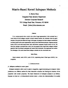
where M is the effective number of channel taps, hijp (t) is the complex valued attenuation weight for the pth path, and τijp (t) is the propagation delay for the pth path. Figure 2 depicts the multipath channels between the various users and receiver 0. We assume that the channel parameters vary slowly with time, so that for sufficiently short intervals of time, the channel is approximately a linear time-invariant system given by hij (τ ) =

M X

|hijp |e−jθijp δ(τ − τijp ),

(3)

p=1

where the phase θijp = arg(hijp ) is assumed to be uniformly distributed between 0 and 2π. The tap delays, τijp are modeled as independent uniform random variables over [0, T ]. Without loss of generality, we will estimate the SIR of user 0 at receiver 0. We assume that user 0 transmits a known sequence of L bits called the training sequence, denoted as a0 = [a0,0 a0,1 . . . a0,L−1 ]T . Let {a1 a2 , . . . . aK } be the set of symbol sequences transmitted by the other K users. The received signal at receiver 0 is matched filtered to the code sequence of user 0 and the output of this filter is sampled every T seconds. We assume that the dominant multipath of the user 0’s signal is perfectly synchronized to the receiver 0. The various multipaths of the interference as well as the weak multipaths of user 0’s signal are not synchronized with receiver 0 and arrive at receiver 0 with some offset delay. In general, the sampled received signal in the mth interval will contain a part of the (m − 1)th symbol as well as a part of the mth symbol of each interfering user. If the received signal at receiver 0 is denoted by x(t), it can be written as x(t) =

K X M X

hj0p

K X M X

j=0 p=1

aj,m−1 sj (t − (m − 1)T − τj0p )

m=0

j=0 p=1

+

L−1 X

hj0p

L X

aj,m sj (t − mT − τj0p ) + n(t)

(4)

m=1

Then, the output of the filter matched to s0 (t), can be written compactly in vector-form as y=

(al0 r l00

+

ar0 r r00 )h00

+

K X

(alj r lj0 + arj r rj0)hj0 + n,

(5)

j=1 l l l where r lj0 = [rj01 rj02 . . . rj0M ] represents the crosscorrelation between s0 (t) and the left

portion of sj (t). This correlation value is a function of the corresponding multipath delay and 4

is given as l rj0p

=

Z

(m+1)T

mT

s0 (t − mT )sj (t − (m − 1)T − τj0p )dt.

(6)

Similarly, the crosscorrelation between s0 (t) and the right portion of sj (t) is r rj0p

=

Z

(m+1)T

mT

s0 (t − mT )sj (t − mT − τj0p )dt.

(7)

If the first multipath of the user 0’s signal is considered to be the dominant one, then since it r l is perfectly synchronized to the receiver, r001 = 1 and r001 = 0. The vector of channel taps in

(5) is given as hij = [hij1 hij2 . . . hijM ]T ,

(8)

and the transmitted symbols due to the interferers are arj = [aj,0 aj,1 aj,2 . . . aj,L−1]T

(9)

alj = [aj,−1 aj,0 aj,1 . . . aj,L−2]T

(10)

The receiver noise n is modeled as an independent zero-mean, complex Gaussian random process with second order moments 2 E[n(k)nH (l)] = σN Iδkl

;

E[n(k)nT (l)] = 0,

(11)

2 where xH denotes the Hermitian transpose of x, σN is the noise power, δlk represents the

Kronecker delta function with l and k denoting the sampling time instants and I is the identity matrix. Note here that we have assumed that the channel taps do not vary over L symbols. We assume that the received bits from the interferers are uncorrelated and mutually uncorrelated, i.e., E[aj,m aj,n] = E[aj,m ]E[aj,n] = 0, for all m 6= n, and j, k = 1, 2...K. The channel taps of the various users are assumed to be uncorrelated as well. Therefore, E[hj0m hj0n ] = 0, for all m 6= n. Further, we assume that the channel is a Rayleigh fading channel, i.e., the impulse response hij (t) is modeled as a zero-mean complex Gaussian random process, in which case the envelope |hij (t)| at any instant is Rayleigh distributed [15]. We now focus our attention on the covariance matrix R, of the observation vectors, that will be used to derive the subspace based SIR estimator. The matrix R can be expressed as R = E[yyH ] = RS + RI + RN ,

(12)

where the above decomposition follows from the assumption of uncorrelated users. In (12), the signal covariance matrix RS is given by rH rH lH lH RS = E[(al0 rl00 + ar0 r r00 )h00 hH 00 (r 00 a0 + r 00 a0 )]

5

(13)

The matrix RS is, in general, a matrix of some rank d ≤ L. As a special case, it can be shown that for a perfectly synchronous system, d would be equal to 1. The noise covariance 2 matrix matrix RN in (12) is given as RN = σN I, and the matrix RI in (12) is the interference

covariance matrix given by 

RI = E 

K X

(alj rlj0 + arj r rj0 )hj0

j=1

K X i=1



lH lH rH rH  hH i0 (r i0 ai + r i0 ai )

(14)

2 Denoting E[hj0p hH j0p ] = σj0p , and under the assumption that the code sequences of the various

interferers are uncorrelated pseudorandom sequences, the matrix RI can be written as 

RI =

 α            

β

0

β

α

β

0 .. .

β



··· 0  

··· 0    .. , . α    ... ... β  

0 ··· ···



β

α

(15)



which is a tridiagonal, symmetric, positive definite matrix with elements α and β given by −1 K X M X 2 1 NX 2 + σj0p c [k]c [k + 1] 0 0 3N 3N 2 k=1 j=1 p=1

!

α=

X K X M 1 2 σj0p c [1]c [N] β= 0 0 6N 2 j=1 p=1 

(16) (17)

The details of the above derivation are shown in the Appendix. It is seen from (17) that the off-diagonal terms β −→ 0 , as N becomes large, since in any practical system, the number of interferers, K ≪ N 2 . Note that the total interference power, σI2 is given by σI2

=

K X M X

r l E[(rj0p + rj0p )2 ] · E[hj0p hH j0p ]

j=1 p=1

= α + 2β

(18)

We can rewrite RI as RI = αI + βT

(19)

where T is given by 

T =

            

0

1

0

1

0

1

0 .. .

1



··· 0  

··· 0    .. . . 0    ... ... 1  

0 ··· ··· 6



1

0



(20)

For large N, β is found to be negligible and RI is approximately diagonal with the diagonal elements equal to the interference power σI2 . Hence we can write RI ≈ σI2 I

(21)

Note that if we had synchronous transmission, i.e. if all the users were perfectly synchronized to user 0’s receiver, then RI would be diagonal. The non-diagonal nature of the interference covariance matrix is a result of the asynchronism in the system - the energy of each interfering bit is spread over two consecutive sampling intervals. The tridiagonal nature of the interference covariance matrix arises from the fact that we considered the maximum offset delay of the transmitted bit sequence of the interferers to be one bit with respect to the training sequence. This is a reasonable assumption, but in the general case where the maximum offset is more than one bit, we would have non-zero terms in the corresponding off-diagonals as well. Then the matrix would no longer be tridiagonal. But as has been shown above, these terms would approach zero for large N. Hence in any case for a large processing gain, RI would be approximately diagonal, with the diagonal elements equal to the interference power.

3

Subspace Based SIR Estimators

3.1

SIR Estimation using Eigenvalue Decomposition (ED)

Given the above formulation for the covariance matrix R, we now use a subspace based approach to arrive at the SIR estimator. To estimate the SIR, we need to separate the desired signal and the interference plus noise signal from the observation vector. In order to separate the signal covariance matrix from the interference plus noise covariance matrix we require the interference plus noise covariance matrix to be proportional to the identity matrix. Following the discussion of Section 2, we see that R can be written as 2 ˜ S + σ˜I+N I, R=R

(22)

˜ S = RS + βT and σ˜ 2 = (σ 2 − 2β + σ 2 ) = (σ 2 − 2β). where R I+N I N I+N ˜ S would in The signal covariance matrix RS is a matrix of some rank d. The rank of R general be different from the rank of RS . As we have already pointed out in Section 2, for 2 2 ˜ S ≈ RS and σ large processing gain, the value of β is negligible leaving us with R ˜I+N ≈ σI+N . 7

˜S Also for negligible β there is no significant change in the value of d and the eigenvalues of R would be approximately the same as those of RS . In order to separate the signal and interference subspaces, an eigenvector decomposition of R results in R = U ΣU H ,

(23)

where U = [e1 . . . eL ] consists of the orthonormal eigenvectors of R. The diagonal matrix, Σ =diag(λi), contains the corresponding eigenvalues, where λ1 ≥ λ2 ≥ . . . ≥ λL . The eigenvalues of R have the following structure [16]       

λi =      

2 σS2 i + σI+N , if 1 ≤ i ≤ d

, 2 σI+N ,

(24)

d+1≤i≤L

where σS2 i is the power (variance) of the desired signal along the ith eigenvector. From (24), we realize that the d largest eigenvalues in Σ correspond to the signal subspace. Further from the results shown in the previous section, the interference covariance matrix RI is almost diagonal. Thus, if we know the dimension d, then the signal subspace can be identified. Then, using (24), we can obtain the powers of the desired signal and the interference plus noise, respectively. This is the basic idea underlying our estimation technique. The true covariance matrix R is of course not known and has to be estimated. Since we want to track time variations of the SIR, we form a moving average or Bartlett estimate of the covariance matrix from the J most recent observation vectors. Let y(k) denote the k th ˆ observation vector. The sample covariance matrix, R(n), after the nth observation vector is formed as 1 ˆ R(n) = J

n X

y(k)(y(k))H

(25)

k=n−J+1

It has been shown, e.g. [17], that the eigenvalues of the sample covariance matrix in (25) is a maximum likelihood estimate of the eigenvalues of the true covariance matrix R. Almost all existing approaches to the determination of the dimension of the signal subspace are based on the observation that the smallest eigenvalue of the covariance matrix has multiplicity L − d. We have tested two information theoretic approaches, both proposed in [18], the Akaike’s Information Criterion (AIC) and the Minimum Descriptive Length (MDL) principle. For our application, both the criteria achieved satisfactory performance. The MDL 8

criterion has been found to obtain superior performance in some cases [11] and further, strong consistency of the MDL method has also been proven in [19]. ˆ1 ≥ · · · ≥ λ ˆ L denote the eigenvalues of the To describe the MDL estimation method, let λ sample covariance matrix in (25). Further, define the sphericity test function, Tsph (d), as P ˆi (L − d)−1 Li=d+1 λ   Tsph (d) = QL 1/(L−d) ˆ λ ) i=d+1 i h

i

(26)

and the MDL objective function, FMDL (m), as

1 FMDL (m) = J(L − m)log[Tsph (m)] + m(2L − m)log(J). 2

(27)

The signal subspace dimension is then estimated as the argument of the following minimization problem [18] dˆ = arg min FMDL (m) . m

(28)

Using (23),(24) (25) and (28) we propose the following subspace based SIR estimation algorithm. Subspace Based SIR Estimator using ED ˆ (1) Make an eigenvector decomposition of the sample covariance matrix R ˆ=U ˆΣ ˆU ˆ H, R ˆ i ), with λˆ1 > . . . > λˆL . ˆ = diag(λ where Σ ˆ using (26),(27) and (28). (2) Estimate the current dimension of the signal subspace, d, (3) Estimate the interference power according to 2 σ ˆI+N =

L X 1 ˆj , λ L − dˆ j=d+1 ˆ

and the signal power according to ˆ

σ ˆS2

=(

d X

j=1

9

2 ˆ j ) − dˆσ λ ˆI+N .

(4) The estimate of the SIR is then obtained as γˆ =

1 σ ˆS2 , 2 Lσ ˆI+N

(29)

where the factor 1/L accounts for the fact that we have L samples (symbols) of the received signal within each observation vector. We derive analytical bounds on the performance of the ED estimator in Section 4 and present numerical results in 5

3.2

Subspace tracking using the PASTd algorithm

The ED estimator described in the previous section is based on eigenvector decomposition which is a computationally intensive task. In the context of a constantly varying channel, the ED estimator may be unsuitable for tracking the SIR. A number of adaptive algorithms for subspace tracking have been developed in the past. Most of these methods can be grouped into three families. In the first one, classical batch ED/SVD methods like the QR algorithm, Jacobi rotation and the power iteration have been modified for use in adaptive processing [20–23]. In the second family, variations of Bunch’s rank-one updating algorithm [24] have been proposed. The third class of algorithms considers the ED/SVD as a constrained or unconstrained optimization problem. In [25], the signal subspace has been shown to be the solution of an unconstrained minimization problem and the projection approximation subspace tracking (PASTd) algorithm has been derived for subspace tracking. Let x be a complex valued random vector process with correlation matrix R. Consider the following scalar function h

J(W ) = E k x − W W H x k2

i

= tr(R) − 2tr(W H RW ) + tr(W H RW · W H W )

(30)

with a matrix argument W ∈ C n×d with d < n. Here, tr(·) is an abbreviation for the trace. In [25] it was proven that J(W ) has a global minimum at which the column space of W equals the signal subspace. At each stationary point of J(W ), it equals the sum of the eigenvalues of those eigenvectors which are not involved in the signal subspace. All sample vectors available in the time interval 1 ≤ t ≤ n are involved in estimating the signal subspace at the time instant

10

Choose cj (0) and wj (0) FOR t = 1, 2, . . . DO y(t) : Current data vector v 1 (t) = y(t) FOR j = 1, . . . d DO xj (t) = wH j (t − 1)v j (t) cj (t) = ρcj (t − 1) + |xj (t)|2 ej (t) = v j (t) − wj (t − 1)xj (t) wj (t) = wj (t − 1) + ej (t)[x∗j (t)/cj (t)] v j+1 (t) = v j (t) − wj (t)xj (t) Table 1: The PASTd algorithm for tracking the signal subspace

n. So, if y(n) is the data input at the nth instant, the cost function to be minimized is, J(W (n)) =

n X

ρn−t k y(t) − W (n)W H (n)y(t) k2

(31)

t=1

where ρ is a forgetting factor meant to downweigh the past observations. The function J(W ) is a fourth order function of the elements of W . Iterative algorithms are thus necessary to minimize J(W ). The PASTd algorithm has been summarised in Table 1. Here, as before, d is the signal subspace dimension and it is assumed to be known. Also, wj (t), j = 1 . . . d are columns of the matrix W (t), and a simple initial choice for these columns would be the d leading unit vectors of the L × L identity matrix, where L is the dimension of the input data vector y. Note that the PASTd algorithm allows for explicit computation of the eigencomponents. To be specific, wj (t) is an estimate of the j th eigenvector of the covariance matrix C(t) and cj (t) is an estimate of the corresponding eigenvalue at time t. Thus, cj (t) = σ ˆS2 j for j = 1, . . . d. The key issue of this approach is to approximate W H (n)y(t) in (31) by the expression x(t) = W H (t − 1)y(t)

(32)

This results in the modified cost function ′

J (W (n)) =

n X

ρn−t k y(t) − W (n)x(t) k2

t=1

11

(33)

The difference between W H (n)y(t) and W H (t − 1)y(t) is small, particularly when t is close to n. The updating of the columns of the W (t) matrix has been indicated in step 4 of ′

the table, where e(t) is an estimator of the gradient of J w.r.t. W (t). The last equation in the table denotes the deflation technique. The basic idea of the deflation technique is the sequential estimation of the principal components [26,27]. First, the most dominant eigenvector is updated using the algorithm with d = 1. Then we remove the projection of the current data vector y(t) onto this eigenvector from y(t) itself. Now since the second dominant eigenvector becomes the most dominant one in the updated data vector (represented by the dummy variable v(t)), it can be extracted in the same way as before. Applying this procedure repeatedly, all desired eigencomponents are estimated sequentially. ′

Further, since J ((W (n)) equals the sum of the noise plus interference eigenvalues at its 2 minimum, we can use it as an estimate of the same, i.e, (L − d)ˆ σI+N . The complexity of

the PASTd algorithm is 4Ld + O(d) operations per update. This is a much lower complexity compared to the ED estimator, since no matrix inversion operations are involved. The performance results of this subspace tracking algorithm are presented in Section 5. While both the ED and PASTd estimators require knowledge of the dimension of the signal subspace, the PASTd algorithm is attractive in the context of time varying SIRs as would be encountered in real cellular systems. Thus, the PASTd algorithm could be initialized using the ED algorithm following which it can execute the subspace tracking mode of SIR estimation.

4

Analysis of the ED Estimator

In order to derive analytical expressions for the accuracy of the ED estimator described in the previous section, we need the following preliminaries. Consider the problem of estimating the covariance matrix of an m−variate normal distribution Nm (µ, C), where, µ is the mean and C is the covariance matrix of the distribution. In this case, the sample covariance matrix S formed from n random vectors X 1 . . . X n has m distinct eigenvalues l1 > . . . > lm which are estimates of the eigenvalues λ1 ≥ . . . ≥ λm of C [17]. Then, it has been shown by Lawley [28] that if λi is a distinct eigenvalue of C, then the mean and variance of li can be expanded for large n, where n is the number of samples, as

12

E(li ) = λi + and

m λj λi X + O(n−2 ) n j=1,j6=i λi − λj





2λ2 1 X λj Var(li ) = i 1 − )2  + O(n−3 ) ( n n j=1,j6=i λi − λj

(34)

(35)

We propose to use the above result for analyzing the accuracy of the SIR estimator. The eigenvalue estimation of the covariance matrix R is equivalent to a sample estimate based on samples from an L−variate normal distribution NL (0, R). 2 The matrix R has (d + 1) distinct eigenvalues, specifically, λi = σS2 i + σI+N for i = 1, . . . , d 2 and λd+1 = σI+N . The eigenvalue λd+1 is a repeated eigenvalue of multiplicity L − d. Note

that the eigenvalues λi , i = 1, . . . , d can be written as λi = σS2 i + λd+1 . Also let us denote γi =

2 σS

i

2 σI+N

. Then, we can write λi = λd+1 (γi + 1)

i = 1, . . . , d.

(36)

ˆ1 . . . λ ˆ L , we can simplify (34) ˆ is the sample covariance matrix, with eigenvalues λ Hence, if R to write 



L γj + 1 γi + 1 X L−d  E(λˆi ) = λd+1 γi + 1 + ( + ) , ∀ i = 1 ... d n j=1,j6=i γi − γj γi

and ˆ d+1 ) = λd+1 E(λ Note that the true SIR is γ =

1 L

Pd

i=1

d 1X 1 1 , 1− − n n i=1 γi

#

"

(37)

(38)

γi . From (29), the estimated SIR is

1 γˆ = L

ˆ −λ ˆ d+1 ) ˆ d+1 λ

Pd

i=1 (λi

!

(39)

Therefore, the expression for the expected value of the estimated SIR is 1 E(ˆ γ) = E L

Pd

ˆ −λ ˆ d+1 ) ˆ d+1 λ

i=1 (λi

d 1X 1 ˆ i )E ≈ E(λ ˆ L i=1 λd+1

!

!

−

d L

(40)

ˆ i ’s and λ ˆ d+1 are independent random Note that in (40) we are making the assumption that the λ variables. We will validate the analysis based on this assumption through numerical results in

13

the next section. Since 1/X is a convex function for strictly non-negative X, applying Jensen’s inequality we bound (40) as P ˆi) d 1 E( di=1 λ E(ˆ γ) ≥ − ˆ d+1 ) L E(λ L

(41)

As a special case, when d = 1 (i.e., when we consider the weak multipaths of the signal as interference and ignore them), the matrix R, has 2 distinct eigenvalues, specifically, λ1 = 2 2 LσS2 + σI+N and λ2 = σI+N . The eigenvalue λ2 is a repeated eigenvalue of multiplicity (L − 1).

For this case, it follows from (41), (37) and (38) that 

E(ˆ γ) ≥ γ + γ 

(n −

3L γ



2 γ2  1)L2 − Lγ

L2 +

+

(42)

The fractional error in the SIR estimate can also be bounded as e=

E(ˆ γ) − γ γ

!

≥

2 γ2 1)L2 − Lγ

L2 + (n −

3L γ

+

(43)

Thus we get lower bounds on the estimator mean and fractional error. For the variance of the above estimator, using (35) it follows that ˆ1 ˆ1 1λ 1 λ 1 Var(ˆ γ ) = Var( − ) = 2 Var ˆ2 L ˆ2 Lλ L λ

!

(44)

ˆ 1 and λ ˆ 2 are independent random variables, and using Jensen’s inequality we Assuming that λ can bound the variance as Var(ˆ γ) ≥

2(Lγ + 1)2 (n(Lγ)2 − 1) (Lγ(n − 1) − 1)2

(45)

It can be seen that as n → ∞, the lower bound on the variance of the estimator → 0. This suggests that the estimate gets increasingly accurate with better averaging, which is to be expected. As an illustration of the tightness of these bounds, consider the case when the signal space dimension is d = 2, and the signal power is equally distributed in both the dimensions. The lower bound on the mean of the SIR estimate can be shown to be 

E(ˆ γ) ≥ γ + γ 

10L γ 2)L2

2L2 +

+

(n −

−



12 γ2  . 4L γ

(46)

Comparing (46) to (42) we notice that for the same γ the lower bound is tighter when the signal space dimension is 1. This is due to the fact that the smaller the signal space dimension, 14

the more accurately can we get an estimate of the interference power by averaging over a larger number of eigenvalues. Consequently, we get a better estimate of the signal power which leads to a better estimate of the SIR. From (41), we note that we always tend to overestimate the SIR. This is due to the fact that we consider the interference covariance matrix to be diagonal and ignore the terms on the off-diagonals. This leads to an underestimation of the interference power, and consequently to an overestimation of the SIR.

5

Numerical Examples

In this section we evaluate the performance of both the ED and PASTd SIR estimators in an hexagonal cellular system. The frame structure used for the numerical examples assumes a reverse traffic channel frame of duration 20ms and operating at 9.6 Kbps. Therefore each frame consists of 192 bits and the frame rate is 50 frames/s. We employ a BPSK modulation scheme with a training sequence of 25 bits. The reason for the above choice of frame length and data rates is to emulate the specifications for an IS-95 system. However, we would like to point out that the choice of the training sequence is purely for illustration and does not conform to the IS-95 specifications. The performance of the estimator is evaluated using the mean, standard deviation and the absolute percentage error as measures. As has been explained in section 3, we form a moving average or Bartlett estimate of the covariance matrix from the J most recent observation vectors. For a fixed SIR, the power transmitted by each user and the channel taps remain the same in each trial. However, the noise samples and the information bits transmitted by the interferers is different in each trial. The mean is formed by averaging the SIR estimates formed from x independent trials. Note that the value of n in equations (34) and (35) is Jx. For simulation purposes, we consider a Rayleigh fading channel with M = 2 taps. The noise floor is taken to be 20dB lower than the transmitted interference level. In Figure 3, we plot the SIR estimated by the ED and the PASTd estimators as a function of the number of frames over which averaging is done, for a fixed SIR of 9 dB. The system considered has K = 3 users and a processing gain of N = 128. The plots are shown for a single trial. We note that both estimators perform quite well. The initial performance of the PASTd estimator depends to some extent on the initial values of the signal eigenvalues that we choose. For the same example, we depict in Figure 4, the mean of the estimated SIR averaged over 100 15

trials, one of which was plotted in Figure 3. Also plotted is the actual SIR and the lower bound on the mean as obtained from the analysis. The lower bound almost exactly equals the actual SIR. The reason for this is the large value of 100 that we have chosen for x in our simulations. The lower bound is highly sensitive to the value of n = Jx. The effect of a large x is essentially to average out the noise. However, our estimation procedure is sensitive largely to J, the number of observed frames. This is because while a large x averages out the noise, the interference is averaged out only when we average over a large number of observed frames. Hence for the estimator, the value of J dictates the performance. For the same example in Figure 5 we plot the standard deviations of both the estimators and the lower bound obtained on the ED estimator from the analysis. We also plot the approximate expression for the standard deviation which was stated in Section 4. We see that standard deviation of the estimators decrease as the estimation time increases. We plot the absolute percentage errors of the estimators in Figure 6. We see that the percentage error of the ED estimator falls to below 20 percent after about 8 frames, and to below 10 percent after less than 15 frames. To study the effect of the processing gain on estimator performance, In Figure 7, we plot the estimator mean and absolute percentage error in Figures 7 and 8, respectively. The plots are shown for processing gains of N=128 and N=256 with the actual SIR being 8.1 dB. As is expected, the mean obtained for the higher processing gain is closer to the lower bound. Also, the difference becomes more significant as the estimation time increases. Recall that the assumption of the interference covariance matrix being diagonal is more valid for larger N. We see that for N=256, the error falls to below 20 percent after 7 frames and to below 10 percent after 11 frames. Thus we have a significant improvement in the performance for a larger processing gain as the estimation time increases. In Figure 9, we plot the error performance of the ED estimator as a function of the observed number of frames for different values of SIR. The system considered has K = 20 interferers and a processing gain of N = 128. The estimates are seen to be good over a wide range of SIR values. In Figure 10, we study the effect of mobile velocity on estimator performance. The starting position of the mobile receiver is uniformly distributed over the cell area. The mobile moves with a constant speed in a direction uniformly distributed in [0, 2π]. In addition to Rayleigh fading, we also consider a shadow fading factor s(t) assumed to be log-normally distributed with a mean of 0 dB, and a log-standard deviation of σf = 8 dB. The shadow fading is further 16

assumed to have to have the time correlation function proposed in [29], which has been derived based on field experimental data. If z(t) = (10/σf ) log10 s(t), then E[z(t + τ )z(t)] = e−vτ /X ,

(47)

where v is the velocity of the mobile user. The parameter X is the effective correlation distance of the shadow fading, and is assumed to be 43 m. We have plotted the percentage error graphs for widely varying mobile velocities. We note that the error curves for all the cases depicted are close to each other proving that the estimator is quite robust to mobile velocities. In Figure 11, we depict the SIR tracking abilities of both the estimators in the context of a constantly time varying SIR. Here the length of the sliding window for the ED estimator J is 20. The value of the forgetting factor ρ for the PASTd estimator is taken to be 0.7. The SIR is plotted as a function of time for more clarity. For this example the SIR variations are quite large. These variations have been achieved by adjusting the power of user 0. Note that the variations can also be achieved by adjusting the interference power. In the practical case of a large number of interferers, on account of the small cross correlation between them, a significant change in the interference power is obtained only if a large number of interferers change their powers significantly. Here the SIR varies every 0.8 sec or equivalently every 40 frames. In Figure 12 we plot the SIR tracking of the estimators for a more rapidly varying SIR again with large SIR variations. The SIR here changes every 0.4 sec, or equivalently every 20 frames. We note that the estimators depict peaks at the points where the SIR changes, but they adapt quite quickly to the changed environment. For the same examples above, we show the mean performance of the estimators averaged over 10 trials in Figures 13 and 14. We note that as the SIR variation becomes more rapid, the performance of both the estimators deteriorate. This is to be expected because the estimators need some time to adapt to the changed SIR and converge to the new value. If the SIR changes before they start converging, they are unable to track the changes effectively. Although, at the transitions points of the SIR, the PASTd estimator exhibits sharp peaks, it adapts quite quickly after that.

6

Conclusions

In this paper we have studied the practical problem of obtaining accurate real time measurements of the SIR for CDMA cellular systems. We have derived a subspace based estimation 17

method, that is based on an eigenvector decomposition of the sample covariance matrix of the received signal. We have also looked at a less complex subspace tracking algorithm. We believe that the above approach for SIR estimation can be used in power control and handoff algorithms. The techniques presented here did not require any prior information about the channel. We have shown via analytical bounds and numerical examples that the ED based SIR estimator is able to estimate the true SIR within an error of 10 percent after an observation interval of only about 11 frames for a processing gain of 256 and an observation interval of less than 15 frames for a processing gain of 128. The subspace method was shown to be relatively insensitive to the actual SIR values or mobile speeds. Our examples show that both the ED estimator and the PASTd estimator are able to track variations in the SIR reasonably well with the PASTd estimator performing slightly better than the ED estimator, especially with good initialization. One approach could be to use the ED estimator to obtain an estimate of the signal space dimension as well as estimates of the covariance matrix eigenvalues with which to initialize the PASTd estimator after which the PASTd estimator could be made to track the SIR. Another attractive feature of the subspace based technique is that it allows easy integration into the multiuser architectures like the MMSE and the decorrelator [30] which are essentially based on projecting the received signal onto a subspace orthogonal to that of the interference (plus noise) subspace. Yet another feature that makes the proposed SIR estimation technique desirable is that it allows for easy implementation on existing VLSI hardware and DSP devices. Also as this technique does not require knowledge about the code sequences of the interfering users, we believe that it can be used for SIR estimation on the forward link as well as the reverse link.

Appendix Derivation of RI Let us define matrices U and L where L = U T and 

 0 0 .... 0    1 0 .... 0

L=    

0 1 .... 0 0 .. 18

1

0

         

(48)

The matrix RI from (14) can now be simplified as RI = E[

K X

(alj r lj0 + arj r rj0 )hj0

j=1

=

RllI

+

K X

lH lH rH rH hH i0 (r i0 ai + r i0 ai )]

i=1

Rlr I

+

Rrl I

+

where

Rrr I ,

(49)

K X

lH r lj0hj0 hH j0 r j0 ]I

(50)

K X

rH r lj0 hj0hH j0 r j0 ]L

(51)

K X

lH r rj0 hj0hH j0 r j0 ]U

(52)

K X

rH r rj0hj0 hH j0 r j0 ]I

(53)

RllI = E[

j=1

Rlr I = E[

j=1

Rrl I = E[

j=1

Rrr I

= E[

j=1

Using the above formulation and by virtue of the assumptions about the channel taps of the various users being uncorrelated, we can write RI in the form of a symmetric tridiagonal matrix as in equation (15) where α=

K X M X

r l E[(rj0p )2 + (rj0p )2 ] · E[hj0p hH j0p ]

(54)

r l E[rj0p rj0p ] · E[hj0p hH j0p ]

(55)

j=1 p=1

β=

K X M X

j=1 p=1

We now proceed to simplify the terms α and β in the above interference covariance matrix. l r Consider the correlation terms, rj0p and rj0p . In any sampling interval nT to (n + 1)T , we have

a part of the present symbol aj,n for every user j, and a part of the previous symbol aj,n−1 (see Figure 1). Suppose, for the j th user, in the pth multipath, we have (m − 1) complete chips and part of the mth chip of an in the given interval. Then, T − τj0p = (m − 1)Tc + tl

(56)

where tl is that part of the mth chip which is in the nth interval, and tr = Tc − tl is the part of the chip which will fall in the next interval. Similarly, in the given interval we will have a l part of the mth chip and (N − m) complete chips of the previous symbol. Then, rj0p can be

written as l rj0p =

−m 1 NX c0 [i](cj [m + i − 1]tr + cj [m + i]tl ) + c0 [N − m + 1]cj [N]tr , T i=1

19

(57)

th n sampling interval nT

(n+1)T

Offset delay τ

tl T

c

tr

Part of the previous Part of the current symbol a n

symbol a n-1

Figure 1: Illustrative example with N=5, and m=4 where the RHS of the above equation is divided by T = NTc in order to normalize the r correlation terms. Similarly, rj0p can be written as r rj0p =

N X 1 c0 [N − m + 1]cj [1]tl + c0 [i](cj [m + i − 1 − N]tr + cj [m + i − N]tl ). T i=N −m+2

(58)

The code sequence of the desired user is either known or deterministic, while those of the other users are pseudorandom sequence. Therefore E[cj [k]] = 0, ∀k, ∀j = 1, 2, ...K. Further, since the chips are independent of each other E[cj [i]cj [p]] = 0, ∀i 6= p. Recall that we had modeled the multipath delays τj0p ’s as uniform random variables ∈ [0, T ] implying that tr and tl are uniform random variables ∈ [0, Tc ]. Therefore E[tr tl ] = Tc2 /6, and E[t2r + t2l ] = 2Tc2 /3. Using the above conditions and equations (57) and (58), it can be shown that 1 Tc2 = c0 [1]c0 [N] 2 ∀ p, j, 2 6T 6N

(59)

−1 2 1 NX + c0 [k]c0 [k + 1]. 3N 3N 2 k=1

(60)

−1 K X M X 1 NX 2 2 σj0p + c [k]c [k + 1] 0 0 3N 3N 2 k=1 j=1 p=1

(61)

l r E[rj0p rj0p ] = c0 [1]c0 [N]

and l r E[(rj0p )2 + (rj0p )2 ] =

2 Denoting E[hj0p hH j0p ] = σhj0p , the terms in RI can thus be written as

!

α=

X K X M 1 2 σj0p c0 [1]c0 [N] β= 2 6N j=1 p=1 

20

(62)

References [1] S. Ariyavisitakul “SIR-based power control in a CDMA system”. In IEEE Global telecommunications Conference, 1992, pp.868-873. [2] R. Beck and H. Panzer. “Strategies for Handover and Dynamic Channel Allocation in Micro-Cellular Mobile Radio Cellular Systems”. In Proc. IEEE 39th Vehicular Technology Conference, pp. 742-748, San Francisco, CA., May 1989. [3] E. A. Frech and C. L. Mesquida. “Cellular Models and Hand-off Criteria,” IEEE Vehicular Technology Conference”, pp. 128-35, 1989. [4] J. Zander. “Performance of Optimum Transmitter Power Control in Cellular Radio Systems”. IEEE Trans. on Vehicular Technology, Vol. 41, No. 1, Feb. 1992. [5] R. D. Yates. “A Framework for Uplink Power Control in Cellular Radio Systems”. IEEE JSAC, Vol. 13, No. 7, Sep. 1995. [6] S. Kozono. “Co-channel Interference Measurement Method for Mobile Communication”. IEEE Trans. on Vehicular Technology, Vol. 36, pp. 7-13, 1987. [7] S. Yoshida, A. Hirai, G. L. Tan, H. Zhou and T. Takeuchi. “In-Service Monitoring of Multipath Delay-Spread and C/I for QPSK Signal”. In Proc. IEEE 42nd Vehicular Technology Conference, pp. 592-595, Denver, CO., Apr. 1992. [8] A. L. Brand˜ao, L. B. Lopez and D. C. McLernon. “Cochannel Interference Estimation for M-ary PSK Modulated Signals” Wireless Personal Communications, Vol. 1, No. 1, pp. 23-32, 1994. [9] A. L. Brand˜ao, L. B. Lopez and D. C. McLernon. “Quality Assessment for Pre-Detection Diversity Switching”. In Proc. PIMRC’95, pp. 577-581, Toronto, Canada, Sep. 1995. [10] M. D. Austin and G. L. St¨ uber. “In-Service Signal Quality Estimation for TDMA Cellular Systems”. In Proc. PIMRC’95, pp. 836-840, Toronto, Canada, Sep. 1995. [11] M. Andersin, N. B. Mandayam, and R. D. Yates, “Subspace based SIR Estimation for TDMA Cellular Systems,” in Wireless Networks, vol. 4, no. 3, pp. 241-247, April 1998. [12] M. Turkboylari and G. L. St¨ uber. “An Efficient Algorithm for Estimating the Signal-toInterference Ratio in TDMA Cellular System,” in IEEE Trans. on COM, vol. 46, no. 6, pp. 728-731, June, 1998. [13] A. M. Viterbi and A. J. Viterbi, “Erlang Capacity of a Power Controlled CDMA System,” in IEEE JSAC, vol. 11, no. 6, pp. 892-900, August, 1993. [14] EIA/TIA Interim Standard-95, ‘Mobile Station — Base Station Compatibility Standard for Dual-Mode Wideband Spread Spectrum Cellular Systems,’ July 1993. [15] J. Proakis. Digital Communications. McGraw-Hill, second ed., 1989. [16] S. Haykin, J. Litva and T. J. Shepherd. Radar Array Processing, Springer Series in Information Sciences, Vol.25, Springer-Verlag Berlin, Heidelberg 1993. [17] R. Muirhead. Aspects of Multivariate Statistical Theory. New York: John Wiley and Sons, 1982. [18] M. Wax and T. Kailath. “Detection of Signals by Information Theoretic Criteria”. IEEE Trans. on ASSP, ASSP-33(2), pp. 387-392, Apr. 1985.

21

[19] L. C. Zhao, P. R. Krishnaiah and Z. D. Bai. “On Detection of the Number of Signals in Presence of White Noise”. Journal of Multivariate Analysis, 20:1:1-25, 1986. [20] P. Comon and G. H. Golub. “Tracking a few extreme singular values and vectors in signal procesing”. Proc. of IEEE, pp. 1327-1343, Aug. 1990. [21] N. L. Owsley. “Adaptive data orthogonalization” Proc. IEEE ICASSP, pp. 109-112, 1078. [22] K. C. Sharman. “Adaptive algorithms for estimating the complete covariance eigenstructure” in Proc. IEEE ICASSP , pp.1401-1404, Tokyo, Japan, Apr. 1986 [23] M. Moonen, P. Van Dooren and J. Vandewalle. “Updating singular value decompositions: A parallel implementation .” in Proc. SPIE Adv. Algorithms Architectures Signal Processing, pp. 80-91, Aug. 1989, San Diego, CA. [24] R. Bunch, C. P. Nielsen and D. Sorenson. “Rank-one modification of the symmetric eigenproblem.” Numerische Mathematik, vol 31, pp. 31-48, 1978. [25] B. Yang. “Projection Approximation Subspace Tracking”. IEEE Trans. on Signal Processing, Vol.43, pp. 95-107, Jan. 1995. [26] J. Yang and M. Kaveh. “Adaptive eigenspace algorithms for direction or frequency estimation and tracking”. Proc. IEEE Trans. Acoust.,Speech.,Signal Processing, vol. 36, pp. 241-251, 1988. [27] S. Bannour and M. R. Azimi-Sadjadi. “An adaptive approach for optimal data reduction using recursive least squares learning method.” Proc. IEEE ICASSP, pp. 11297-11300, Mar. 1992, San Francisco, CA. [28] D. N. Lawley “Tests of significance for the latent roots of covariance and correlation matrices.”Biometrika, 43, pp.128-136, 1956. [29] M. Gudmundson. “Correlation Model for Shadow Fading in Mobile Radio Systems.” Electronic Letters, Vol. 27, No. 23, pp. 2145-2146. Nov. 1991. [30] X. Wang and H. V. Poor. “Blind Adaptive Interference Suppression for CDMA Communications Based on Eigenspace Tracking.” Proceedings of CISS, Baltimore, MD, March 1997.

22

s0 (t)

User

Σ

h000

0

x(t)

( ) dt

h00M

y

Receiver 0

h101

1

h10M

hK01

hK0M K

Figure 2: System model - Multipath channels between the various users and the receiver 0

A sample path for the estimators 11 Actual SIR ED Estimator PASTd Estimator

10

SIR in dB

9

8

7

6

5

4

0

10

20

30

40 50 Number of frames

60

70

80

Figure 3: SIR estimate of the two estimators vs. number of frames observed - single trial

23

N=128, K=3, M=2 11 Actual SIR ED Estimator 10

PASTd Estimator Lower bound for ED Estimator

SIR in dB

9

8

7

6

5

4

0

10

20

30

40 50 Number of frames

60

70

80

Figure 4: Mean SIR of the estimators and the analytical lower bound of the ED estimator vs. number of frames observed

N=128, M=2, K=3 6 ED estimator Lower bound for ED Estimator Approximation for ED Estimator PASTDd Estimator

5

Standard Deviation

4

3

2

1

0

0

10

20

30

40 50 Number of frames

60

70

80

Figure 5: Standard Deviation of the estimators and the analytical lower bound of the ED estimator vs. number of frames observed 24

N=128, M=2, K=3 70 ED Estimator PASTd Estimator 60

Absolute Percentage Error

50

40

30

20

10

0

0

10

20

30

40 50 Number of frames

60

70

80

Figure 6: Percentage error of the estimators vs. number of observed frames

M=2, K=3 10.5 Actual SIR ED Estimate for N=128 ED Estimate for N=256 10

SIR in dB

9.5

9

8.5

8

0

5

10

15

20 25 Number of frames

30

35

40

Figure 7: Mean of the ED estimator for different processing gains as a function of the number of observed frames

25

M=2, K=3 70 Error for N=128 Error for N=256 60

Absolute Percentage Error

50

40

30

20

10

0

0

5

10

15

20 25 Number of frames

30

35

40

Figure 8: Absolute percentage error of the ED estimator for different processing gains as a function of the number of observed frames N=128, K=20, M=2 Averaging done over 20 trials 60 SIR=1.5 dB SIR=3.6 dB SIR=6.5 dB

50

Absolute percentage errors

SIR=9dB

40

30

20

10

0

0

10

20

30

40 50 Number of frames

60

70

80

Figure 9: Percentage error of the ED estimator vs. number of observed frames for different values of the SIR for 20 interferers 26

N=128, K=20, M=2

Averaging done over 20 trials

40 v=5 km/h v=50 km/h v=90 km/h

35

Absolute Percentage Error

30

25

20

15

10

5

0

0

10

20

30

40 50 Number of frames

60

70

80

Figure 10: Percentage error of the ED estimator vs. number of observed frames for different mobile velocities

N=128, K=3, M=2

Sample paths of the estimators

11.5 Actual SIR ED Estimator PASTd Estimator

11

10.5

SIR in dB

10

9.5

9

8.5

8

7.5

7

0

0.5

1

1.5 2 Time in seconds

2.5

3

3.5

Figure 11: Tracking ability of the estimators for a time varying SIR

27

N=128, K=3, M=2

Sample paths of the estimators

12 Actual SIR ED Estimator PASTd Estimator

11

SIR in dB

10

9

8

7

6

5

0

0.5

1

1.5 2 Time in seconds

2.5

3

3.5

Figure 12: Tracking ability of the estimators for a more rapidly time varying SIR

N=128, K=3, M=2

Estimator mean after 10 trials

11.5 Actual SIR ED Estimator PASTd Estimator

11

10.5

SIR in dB

10

9.5

9

8.5

8

7.5

7

0

0.5

1

1.5 2 Time in seconds

2.5

3

3.5

Figure 13: Mean performance of the estimators for the less rapidly varying SIR

28

N=128, K=3, M=2

Estimator mean after 10 trials

12 Actual SIR ED Estimator PASTd Estimator

11

SIR in dB

10

9

8

7

6

0

0.5

1

1.5 2 Time in seconds

2.5

3

3.5

Figure 14: Mean performance of the estimators for the more rapidly varying SIR

29