and noise-free low resolution images were originally sampled from a ... trattanapachich and Bose presented a spatial domain ... can deal with irregular registration after a process of stamping ... found in the image as well as in the registration.
Super-resolution Fusion using Adaptive Normalized Averaging Tuan Q. Pham
Lucas J. van Vliet
Quantitative Imaging Group, Faculty of Applied Sciences, Delft University of Technology, Lorentzweg 1, 2628 CJ Delft, The Netherlands {tuan, lucas}@ph.tn.tudelft.nl www.ph.tn.tudelft.nl/∼lucas Keywords: super-resolution, sampling density, adaptive normalized averaging, irregular samples
Abstract A fast method for super-resolution (SR) reconstruction from low resolution (LR) frames with known registration is proposed. The irregular LR samples are incorporated into the SR grid by stamping into 4-nearest neighbors with position certainties. The signal certainty reflects the errors in the LR pixels’ positions (computed by cross-correlation or optic flow) and their intensities. Adaptive normalized averaging is used in the fusion stage to enhance local linear structure and minimize further blurring. The local structure descriptors including orientation, anisotropy and curvature are computed directly on the SR grid and used as steering parameters for the fusion. The optimum scale for local fusion is achieved by a sample density transform, which is also presented for the first time in this paper.
1 Introduction Super-resolution from a sequence of low resolution images is an important step in early vision to increase spatial resolution of captured images for later recognition tasks. An extensive literature on this topic exists [1] [2], of which there are two main approaches: one with simultaneous estimation of image registration parameters and the high resolution image [3] [4] and the other with registration being computed separately before fusion [5] [6]. The super-resolution algorithm presented in this paper follows the second approach. In other words, given an estimate of the registration, our method attempts to reconstruct a high resolution image that is visually more informative than each of the individual low resolution frames. The main tasks involved in the fusion process are first to map the irregular pixels onto a rectangularly
sampled SR grid and secondly to derive the SR grid values from them. The first attempt of such was initiated by Tsai and Huang [7], who assumed the aliased and noise-free low resolution images were originally sampled from a band-limited high resolution image. Kim, Bose and Valenzuela [5] extended this work to handle noisy and blurred LR images using recursive least squares optimization in the Fourier domain. A spatial domain method was then reported by Ur and Gross [8]. However, all these early algorithms only works with shifted LR inputs that can be aligned periodically within the SR grid. In a recent paper [6], Lertrattanapachich and Bose presented a spatial domain method based on Delaunay triangulation [9] that allows any arbitrary organization of input samples. Our structure adaptive fusion algorithm in this paper also can deal with irregular registration after a process of stamping pixels back onto the grid. However, it is much less sensitive to noise than a perfect surface reconstruction algorithm like [6] because of an averaging along the dominant local structure.
The paper is organized as follows: section 2 briefly describes the signal/certainty principle in image processing via normalized averaging. Fusion of irregular and uncertain samples is possible under this principle by using 4-nearest neighbor stamping of the signal certainty. Section 4 introduces the density transform to compute sampling density of a set of irregular pixels. Section 5 combines adaptive filtering and density transform into the normalized averaging equation to achieve a structure-enhanced fusion result. Simulations and analysis of the super-fusion technique are given in section 6. Section 7 finally concludes the paper.
2
Normalized Averaging
Normalized Averaging (NA), a special case of Normalized Convolution [10], is a local signal modelling method that takes signal uncertainty into account. The certainty of the signal may reflect noise found in the image as well as in the registration. Using a weighted average with signal certainty contributing to the weights, the method aims at maximizing the reconstructed signal continuity while maintaining the least deviation from the unknown underlying signal in a least squares sense. This characteristic is desirable for various interpolation tasks such as image reconstruction from uncertain data, interpolation and super-resolution. In terms of efficiency, a normalized averaging operation requires only two convolutions (*) with a fixed applicability function a (see equation 1, where s is the input signal, c is the associated certainty and r is the reconstructed signal). This applicability function decides how the neighboring signals influence the local signal model. Generally speaking, any local function that decays outside a certain radius can be used as the applicability function. Amongst those, a Gaussian function is the most popular due to its good localization in both spatial and frequency domain and a fast implementation [11]. r=
(s.c) ∗ a c∗a
(1)
One simple illustration of the signal/certainty principle and normalized averaging is to reconstruct an image from sparse samples. In this example, a signal certainty of one is assigned to the available pixels and zero to the unavailable ones. Note that a simple Gaussian convolution of the degraded signal convey no information; whereas a normalized averaging operation results in a desirable outcome (figure 1). This interpolation result is comparable to a surface reconstruction technique like the Delaunay triangulation method [9] (built-in MATLAB function gridata), but it is much more efficient and robust to noise.
Figure 1: (a) input with only 10% samples, (b) convolution result with a Gaussian kernel σ = 1, (c) normalized averaging result using a Gaussian σ = 1, (d) linear interpolation by Delaunay triangulation.
3 Fusion of Irregular Samples using 4NN Stamping Image fusion of irregularly sampled data is also possible using normalized averaging approach. Difficulties arise, however, because the convolution with
a Gaussian applicability function has to be performed on signal values registered at off-grid positions on the SR grid. In a recent paper, Andersson and Knutsson [12] proposed continuous normalized convolution to approximate the Gaussian spreading of an off-grid sample by truncating the local Taylor expansion up to the first derivative order. The approximation, though fast, does not perform well for small applicability function because of inaccuracy in derivative estimation. Pham and van Vliet [13], in such cases, lookup the filter coefficients from a table and do a direct accumulation of the sample spreading on the SR grid. This method, though more accurate, would induce a lot of computations since each local kernel must be looked up separately. In this paper, we avoid convolution of irregular samples by first stamping those samples with certainties onto the reference SR grid, followed by normalized averaging on the SR grid. The stamping step, which partially assigns an off-grid sample to its four nearest on-grid neighbors (4-NN), divides the certainty into four parts in a bilinear fashion. The stamped signal, weighted with its corresponding certainty share, is accumulated to the weighted sum of signals stored at each pixel (scaccum ). The certainty share is also accumulated to a SR certainty image (caccum ). After every sample has been stamped, normalized averaging takes place on the SR grid as normal with the weighted sum of signals and the SR certainty. This whole process is illustrated in Figure 2. (1-p)(1-q).{s.c,c}
:
p
…
p(1-q).{s.c,c}
q 1-q
(1-p)q.{s.c,c}
SCaccum
1-p
… {s,c}
:
pq.{s.c,c}
ulated
Caccum
}
r=
sc ∗ a c∗a
r
ulated
Figure 2: 4-NN stamping of an off-grid pixel (black point) onto the SR grid (white points), followed by normalized averaging of the accumulated signal and certainty. The accumulation of signal and certainty after the 4-NN stamping is actually a normalized averaging in nature. The bilinear weight distribution could be seen as the result of filtering the irregular sampled input with a bilinear filter. The base width of this filter is twice the pitch of the SR grid and the gray volume under the filter is one. Sampling the filtered input by the SR grid yields a space-variant filtering of the irregular input sample that only affects its 4 nearest neighbors. The smoothing factor of this filter varies but stays below a fraction of the SR grid size. In the worst case scenario when the off-grid pixel is registered halfway in between the SR grid, the space-variant low-pass filter then approximates a 2x2 uniform filter. Due to the
associativity of convolution, the result of normalized averaging on the accumulated signal and certainty is equivalent to normalized averaging on the irregular data with a slightly bigger smoothing sigma. This extra smoothing is however negligible in our superresolution task compared to the blur caused by the optics and the near 100% fill-factor of CCD sensors.
4 Density Transform From the illustration in section 2, it is clear that normalized averaging is an effective method for signal interpolation. However, the quality of the reconstruction depends heavily on the scale of the applicability function. For example, a Gaussian applicability function with a small sigma yields a result similar to nearest neighbor interpolation with undesirable flatpatches effects. A larger Gaussian sigma, on the other hand, incurs excessive blurring to the output, which smooths out the wanted details. More importantly, since the density of the registered samples varies from point to point over the whole SR image, a single scale might introduce unnecessary smoothing over some region while it might not be large enough to cover large gaps in the data. In this section, a method for computing sample density is established. The result could then be used to control the automatic scale selection in the normalized averaging process. The density transform of a gray-scale certainty image is defined as the smallest radius of a pillbox, centered at each pixel position, that encompasses a total certainty value of at least one. The density transform of a SR certainty image (defined in section 3) gives an indication of how dense the SR image is sampled in the vicinity of each pixel. The scale selection for the image fusion process is based on this information to limit the number of contributions from the neighborhood in the normalized averaging process. This ensures a minimum degree of blurring everywhere in the reconstructed image. The density transform is estimated by interpolating responses to a filter bank of increasing radii. By definition, convolution of local image with a pillbox filter of radius equal to the density transform results in a response of one. Pillbox filters with smaller radii thus give responses less than one, and vice versa. The response function therefore increases monotonically with the filter radius. In fact, it could be shown that the response stays zero until the radius reaches a certain value (the distance transform [14]); then, from that point on it keeps increasing with a roughly parabolic shape. A good approximation of the density transform could therefore be computed by piecewise quadratic interpolation. To reduce quantization errors in the pillbox filter, we use a smooth pillbox model based on the cosine function with r0 being the pillbox radius (equation 2).
This smoothing model implies a minimum pillbox radius of 0.5. 1, r ≤ r0 − 0.5; 0, r ≥ r0 + 0.5; hpillbox (r ; r0 ) = (1 + cos(π(r − r0 + 0.5)))/2, otherwise. (2) Apparently, the number of radius samples and the spacings between them determine the accuracy of the algorithm. Depending on the need of the problem, these settings are chosen accordingly. For example, if many LR images are used to construct a SR image, the SR certainty image might be quite densely filled after the 4-NN stamping; accuracy is therefore desired for small density. A sequence with an exponentially increasing step-size such as r0 = 0.5 ∗ 2n/2 (n = 0, 1, 2, ...) could be used in such situation.
5 Adaptive Normalized Averaging If in section 4 we compute a variable scale for the applicability function; in this section, we improve normalized averaging further by applying structure adaptive filtering to the equation. It is clear that LR images often suffer from severe aliasing that causes jaggedness along edges (figure ??b). Normal interpolation algorithms, including the original NA in section 2, reduce these jaggedness by smoothing the edges in all directions, thus also smearing out important details. To avoid such over-smoothing, adaptive filters that are elongated along local orientation are used instead of an isotropic Gaussian kernel in the original NA equation (equation 1). The steering parameters for the adaptive filter is computed from the Gradient Structure Tensor (GST) as follows.
5.1 GST from irregular data Being a least squares estimate of the local gradient vectors, the GST (equation 3) is a reliable orientation estimator. Apart from the orientation (φ), which is the direct result of a principal component analysis on the GST, other important local descriptors such as anisotropy (A) and curvature (κ) can also be derived (equation 4). Anisotropy indicates how strong the edge or line is in the local neighborhood. Curvature is defined as the rate of change of orientation along the dominant linear structure. Note that due to a sudden jump at ±π/2, φ is not directly differentiable. However, we can use the double angle representation in a complex orientation mapping to assure continuity for the differiation [15] [16]. T = ∇I∇I T = λu uuT + λv vvT φ = arg(u)
A = (λu − λv )/(λu + λv )
(3) (4)
u ϕ
v
y = 12 κ x 2
Figure 3: (a) curvature-bent scale-adaptive anisotropic Gaussian kernel, (b) variable density input with adaptive filters, (c) fusion result with missing holes properly filled in. κ = ∂φ/∂v = sin φ · ∂φ/∂x + cos φ · ∂φ/∂y The GST can be constructed from irregular and uncertain data by first stamping the data with certainty onto the SR grid as described in section 3. The image gradients (∇I) can then be computed using Normalized Differential Convolution (NDC) [10] or Derivative of Normalized Convolution (DoNC) [17]. Both techniques are capable of estimating gradient from uncertain data. Although NDC is an optimal estimator in a least-squares sense, DoNC is used in this paper due to its simple implementation and a satisfactory result. The gradient scale used in equation 5 for Gaussian smoothing (g) and derivative (gx ) is 1. The tensor smoothing scale (•) used in equation 3 to compute the GST is 3. ∂ DoN C = ∂x =
5.2
�
(s.c) ∗ g c∗g
�
(5)
(c ∗ g)((s.c) ∗ gx ) − (c ∗ gx )((s.c) ∗ g) (c ∗ g)2
Structure Adaptive Filtering
Local structure adaptive filtering is not a new concept. Several authors [18] [13] have proposed to shape the smoothing kernel after the principal components of the inverse GST. In this paper, we use the same adaptive filtering scheme as in [13]. The filter is a curvature-bent anisotropic Gaussian with its two orthogonal axes aligned with the directions of the GST’s principal components. The scales along these directions are given by equation 6, where C encompasses the local signal-to-noise ratio, α controls the degree of structure enhancement and σdens is the density transform as computed in section 4. In this paper, we use the default value of 1 for both C and α. It is then trivial to see that σu /σv = λv /λu as suggested in [18]. The novel element of this technique is the use of curvature to enable a better fit of the filter to the local linear structure. σu = C(1 − A)α σdens
σv = C(1 + A)α σdens (6)
Although the adaptive filter varies at each pixel position, it needs not be inefficient if a right implementation is used. Rather than rotating, scaling and bending the filter to fit with local image, we do the inverse transformation to the local image instead. The anisotropic Gaussian filter could then be looked up from a coefficient table. Furthermore, if the image contains a lot of linear structures, the filter is contracted in one direction therefore few operations are needed for the direct convolution. For example, our implementation1 of the local structure adaptive filter would take 0.6, 3 and 13 seconds for a 256x256, 512x512 and 1024x1024 image respectively, including time for computing the adaptive parameters.
6 Super-resolution Experiments Every super-resolution algorithm consists of at least two components: image registration and image fusion. With a known registration, the problem reduces to fusion of irregular and uncertain data. The signal irregularity comes from the fact that the scene is captured at different positions in space and time. In fact, the more irregular the data is, the better superresolution result could be obtained. The signal uncertainty comes from the noise of the signal as well as the registration. Registration using optical flow, for example, generates high-confident flow for complex textured regions and low-confident flow for flat regions. Up until now, there are very few superresolution algorithms that incorporate signal certainty into their model. As a result, a single poorly registered frame could totally degrade the output quality. With normalized averaging, however, such disaster could be avoided since we can put less emphasis on these culpable frames. To demonstrate the effectiveness of adaptive normalized averaging for super-resolution, we apply it to two experiments: one with a synthetic sequence and known registration and one with a real sequence taken by a digital camcorder.
6.1 A Synthetic Example In the first experiment, 256x256 super-resolution images are constructed from multiple 64x64 lowresolution images. The LR images are generated from a HR Pentagon scene (1024x1024) using a square sensor model found in common CCD cameras. Difference in image registration is achieved by rotating and translating the scene before a simulated sampling process. Gaussian noise is added to both the gray values and the registered positions. In this experiment, although the registration is known, very few LR frames are available for a 4-time upsampling in 1 C implementation with Matlab interface on an AMD Athlon XP 1.47MHz 1GB RAM
each dimension. Besides the noise, a high fill-factor is also an unnegligible factor in all SR construction algorithms (perfect point resampling with 0% fill-factor is often assumed in many experiments in the literature [6] [5]). Despite many of these poor conditions, the performance of SR using adaptive normalized averaging is superior than surface interpolation using Delaunay triangulation [6]. In figure 5a, under a noiseless condition with a small fill-factor, the two methods perform equally well. As soon as noise is present in both gray values as well as registration (figure 5b), adaptive normalized averaging start to outperforms the other method. The effect of noise is largely diminished thanks to an adaptive regularization along local structures. Furthermore, the oriented regularization also requires fewer LR frames for a visually convincing reconstruction because extra local information such as orientation and curvature are used in the fusion process. These adaptive parameters for the Pentagon experiment with 25% fill-factor under a moderate noisy condition can also be seen in figure 4. To further understand why adaptive normalized averaging is less susceptible to noise than a perfect surface reconstruction method, we need to take a closer look at the input and the adaptive parameters. The Pentagon image is a good image for adaptive fusion since the building contains a lot of linear structures. This fact can be confirmed in the orientation image (fig. 4c), in which there are areas of similar color along each of the five facets of the building. As long as the dominant orientation is known, a 2-D superresolution problem reduces to a single-dimensional reconstruction problem. Four LR frames therefore is enough for a 4-by-4 upsampling as shown in figure 5b. The other two parameters to be looked at are the directional scales σv and σu . Again, the trace of the Pentagon’s five facets is seen in σv , where a darker value means less smoothing across the building edges. The same region in σu image gets brighter, on the other hand, which corresponds to an elongated smoothing to suppress noises along the linear structures. Not only adaptive on the orietation, our SR algorithm also adjusts it fusion process based on sample density. The interwoven pattern on both scale images (fig. 4d-e) is the effect of an automatic scale selection based on local density of LR samples. Black dots in between the pattern suggest a presence of LR samples. These positions get less diffusion compared to other locations with larger gaps in the data. As more LR frames are available with correct registration, the SR certainty image may get filled more evenly and this interwowen pattern may be less noticeable. Finally, the result of SR fusion under an extreme situation such as high-interference radiowave imaging is shown in figure 5c. Ten LRs of 64x64 are synthetically captured by a square CCD array with 100%
fill-factor. High Gaussian noise are added to both intensity (σI = 20) and registration of LR images (σr eg = 0.5 LR pitch). The LR images (fig. 4c) are almost unrecognizable, so does the SR construction using Delaunay triangulation. However, with structure adaptive fusion, valuable structures, such as the path leading into the building, has been successfully recovered.
7 Conclusion In conclusion, we have shown that adaptive normalized averaging is an effective technique for superresolution fusion of image sequences with known registration. The low resolution input samples at irregular positions are incorporated into the super-resolution grid using 4-nearest neighbor stamping with divided sample certainties. Fusion takes place on the superresolution grid by normalized averaging with a structure adaptive applicability. The applicability function is a scale-adaptive, curvature-bent, anisotropic Gaussian that aligns to the local linear structures. The scale of the applicability is derived from the sample density, which minimizes unnecessary blurring in the final fusion. A current limitation of the algorithm is a lack of a built-in deconvolution routine. Our research in the future therefore would be how deblurring could increase the fusion quality, and whether it should be done inline or as a post-processing stage. A modification of the filter shape in the normalized averaging equation is required for such an integration. Under this scheme, it would then be possible to deconvolve spatially variant blur [19], which is commonly found in scenes with a large depth of field.
References [1] P. Cheeseman, B. Kanefsky, R. Kraft, and J. Stutz. Super-resolved surface reconstruction from multiple images. Technical report FIA-9412, NASA, 1994. [2] S. Borman and R.L. Stevenson. Superresolution from image sequences - a review. In Proc. of the 1998 Midwest Symposium on circuits and Systems, volume 5, 1998. [3] M. Irani and S. Peleg. Improving resolution by image registration. CVGIP: Graphical Models and Image Processing, 53(3):231–239, 1991. [4] R.C. Hardie, K.J. Barnard, and E.E. Armstrong. Joint map registration and high-resolution image estimation using a sequence of undersampled images. IEEE Trans. on Image Processing, 6(12):1621–1633, 1997.
a. 64x64 noisy LR input with 25% fill-factor
c. Orientation on SR grid (φ ∈ [−π/2
π/2])
e. Smoothing scale k orientation (σu )
b. very noisy LR input with 100% fill-factor
d. Anisotropy on SR grid (A ∈ [0 1])
f. Smoothing scale ⊥ orientation (σv )
Figure 4: Control parameters for a 4-time SR from 4 noisy 64x64 LR frames in figure a (images are stretched).
a. 4x SR from 20 frames (fill-factor ff = 6.25%, intensity noise σI = 0, registration noise σreg = 0)
b. 4x SR from 4 noisy frames in figure 4a (ff = 25%, σI = 10, σreg = 0.2)
c. 4x SR from 10 very noisy frames in figure 4b (ff = 100%, σI = 20, σreg = 0.5) Figure 5: 4-time super-resolution in each direction from few noisy 64x64 LR frames with noisy registration (σ reg is measured in LR pitch) using Delaunay triangulation (left) and adaptive normalized averaging (right).
[5] S.P. Kim, N.K. Bose, and H.M. Valenzuela. Recursive reconstruction of high resolution image from noisy undersampled multiframes. IEEE Trans. on Acoustics, Speech and Signal Processing, 38:1013–1027, 1990. [6] S. Lertrattanapanich and N.K. Bose. High resolution image formation from low resolution frames using Delaunay triangulation. IEEE TIP, 11(12):1427–1441, 2002. [7] R.Y. Tsai and T.S. Huang. Multiframe Image Resoration and Registration, chapter 7 in: Advances in Computer Vision and Image Processing, pages 317–339. 1984. [8] H. Ur and D. Gross. Improved resolution from subpixel shifted pictures. CVGIP: Graphical Models and Image Processing, 54(2):181–186, 1992. [9] A. Okabe, B. Boots, and K. Sugihara. Spatial tessellations Concepts and applications of Voronoi diagrams. Wiley, 1992. [10] H. Knutsson and C-F. Westin. Normalized and differential convolution: Methods for interpolation and filtering of incomplete and uncertain data. In Proceedings of IEEE CVPR, pages 515– 523, New York City, USA, 1993. [11] I.T. Young and L.J van Vliet. Recursive implementation of the gaussian filter. Signal Processing, 44(2):139–151, 1995. [12] K. Andersson and H. Knutsson. Continuous normalized convolution. In Proceedings of ICME’02, pages 725–728, Lausanne, Switzerland, 2002. [13] T.Q. Pham and L.J. van Vliet. Normalized averaging using adaptive applicability functions with application in image reconstruction from sparsely and randomly sampled data. In Proceedings of SCIA’03, LNCS Vol. 2749, pages 485–492, Goteborg, Sweden, 2003. SpringerVerlag. [14] P.E. Danielsson. Euclidean distance mapping. CGIP, 14:227–248, 1980. [15] G.H. Granlund. In search for general picture processing operator. CGIP, 8(2):155–173, 1978. [16] M. van Ginkel, J. van de Weijer, L.J. van Vliet, and P.W. Verbeek. Curvature estimation from orientation fields. In SCIA’99, pages 545–551, Greenland, 1999. [17] F. de Jong, L.J. van Vliet, and P.P. Jonker. Gradient estimation in uncertain data. In MVA’98, pages 144–147, Makuhari, Chiba, Japan, 1998.
[18] M. Nitzberg and T. Shiota. Nonlinear image filtering with edge and corner enhancement. IEEE Trans. on PAMI, 14(8):826–833, 1992. [19] M-C. Chiang and T.E. Boult. Local blur estimation and super-resolution. In CVPR’97, pages 821–826, Puerto Rico, 1997.