Superresolution Approach of Remote Sensing Images based on Deep

Available online at www.ijpe-online.com

vol. 14, no. 3, March 2018, pp. 463-472 DOI: 10.23940/ijpe.18.03.p7.463472

Superresolution Approach of Remote Sensing Images based on Deep Convolutional Neural Network Jitao Zhanga, Aili Wanga,*, Na Anb, and Yuji Iwahoric a

Higher Education Key Lab for Measure& Control Technology and Instrumentations of Heilongjiang, Harbin University of Science and Technology, Harbin, 150080, China b Hytera Communications Corporation Limited, Harbin, 150001, China c Department of Computer Science, Chubu University, Aichi, Japan

Abstract Nowadays, remote sensing images have been widely used in civil and military fields. But, because of the limitations of the current imaging sensors and complex atmospheric conditions, the resolution of remote sensing images is often low. In this paper, a superresolution reconstruction algorithm based on the deep convolution neural network to improve the resolution of the remote sensing image is proposed. First, this algorithm learned a series of features of the mapping between high and low resolution images in the training phase. This mapping is expressed as a kind of deep convolutional neural network; the trained network is a series of parameter optimization for super-resolution reconstruction of remote sensing image. Experimental results show that the superresolution algorithm proposed in this paper can keep the details subjectively and improve the evaluation index objectively. Keywords: remote sensing image; image superresolution; deep convolutional neural network; parameter optimization (Submitted on December 6, 2017; Revised on January 16, 2018; Accepted on February 12, 2018)

© 2018 Totem Publisher, Inc. All rights reserved.

1. Introduction Remote sensing plays an increasingly important role in mapping and monitoring the Earth. Increasing the availability of high spatial resolution remoting sensing data is an active drive for many remote sensing applications such as urban mapping, military surveillance, intelligence gathering and disaster monitoring. In recent years, the super resolution reconstruction algorithm of remote sensing image has been developed very well. In 2002, H. Tao [9] first used wavelet transform to decompose remote sensing image and get wavelet coefficients through the nearest interpolation, bilinear interpolation and bicubic interpolation. The wavelet transform combined with interpolation algorithm can well maintain the high frequency information to obtain high resolution image. In 2006, [6] proposed a modified inverse iterative projection method for super resolution reconstruction of a group of advanced land observation satellite (ALOS) images, which can effectively deal with the local affine transformation. In 2011, [17] used support vector regression method for learning priori knowledge between the high resolution image and the low resolution ones to get a better model of remote sensing image for super-resolution reconstruction. Single image superresolution (SISR) methods based on external examples learn nonlinear mapping relationship between high resolution (HR) image and low resolution (LR) image from the prior knowledge of a large number of image pairs. Then, the learned function relationship is used to achieve the super resolution reconstruction of the image. Generally, the basic architecture of the SISR method based on the external sample learning is as follows. LR image is first decomposed into LR image blocks overlap in a fixed size. Then, each LR image block proceeds the reconstruction of the corresponding HR image block using mapping learning. Finally, aggregate all HR image blocks overlap to generate high resolution imagery. SISR method based on external sample learning can be classified according to different machine learning methods.

* Corresponding author. E-mail address: aili925@hrbust. edu.cn

464

Jitao Zhang, Aili Wang, Na An, and Yuji Iwahori

Some SISR method based on the external sample learning is used in the joint optimization strategy, which combines the enlargement of the LR image block and the HR image block together. JOR (Jointly Optimized Regressors) studies a series of regression function from a large number of external HR image block and LR image block. It then uses the method of approximate KNN to process each LR image block to choose the best regression function. Learning regression function set selects the best combination of joint optimization function for each LR image block. Joint optimization strategy can effectively improve the performance of SISR method. In 2013, the sparse representation method was introduced to the remote sensing image super resolution reconstruction by Y. Zhang [18]. The overcomplete dictionary is divided into two parts: original dictionary used to obtain the initial high resolution remote sensing image from low resolution images, and residual dictionary used to reconstruct the initial loss of high resolution image information to improve the resolution of the remote sensing image. In order to overcome defects of the traditional sparse representation, which only used one type of feature to reconstruct the remote sensing image, different types of features of various dictionaries were used to obtain texture structure of images in 2015. This algorithm enabled the reconstruction of remote sensing image more accurately. Recently, deep learning is the focus of people’s attention. It is well applied to various fields, such as object recognition and image classification. Practice has proved that the deep learning method can be used to solve the problem of low level vision, such as image deblurring. At the same time, for the SISR, scholars put forward learning framework based on deep learning of end to end which is a major breakthrough. In this paper, the convolutional neural network is introduced into remote sensing image superresolution reconstruction algorithm. Experimental results show that the method can get high resolution image and improve the subjective quality and objective evaluation index [1]. 2. The Basic Theory of Convolutional Neural Network In mid twentieth century, Wiesel and Hubel found a strange network structure of neurons in the cerebral cortex of the cat, that can reduce the complexity of the feedback neural network. Then, they proposed the CNN (Convolutional Neural Network) concept. The use of CNN can be traced back to 1989; in recent years it has become a hot research topic in computer vision [12]. CNN has the following several different characteristic as a special network structure: •

Local perception

Due to the relationship between the image spaces, the pixel correlation of the near distance is relatively high; otherwise, it is low for the far distance. So, the image is a local space in CNN, and each neuron can only feel the local area of the image. Then, as long as these neurons are responsible for different areas in a higher level, the information of the overall situation can be obtained. CNN reduces the number of connections through reducing the number of parameters that need to be trained. •

Weight Sharing

The same convolution kernel is used to convolute all of the hidden layer neurons. This is the concept of weight value sharing. While a convolution kernel is corresponding to feature extraction, a few filters can be added when a variety of features are needed. If 10 kinds of different features are needed, use 10 different filters to convolute the image; the 10 different feature maps of the image can be obtained to form a layer of neurons [11]. In the convolutional neural network, each convolution filter of convolution layer has effects on the receptive field repeatedly. The results of convolution with the input image constitute the feature map of the input image to extract the local features of the image. Each convolution filter shares the same parameters, including the same weight matrix and bias terms as shown in Figure 1. m layer

m-1 layer

Figure1. The Schematic Diagram of Weight Sharing

In the above Figure 1, the m-th layer feature image contains 3 neurons and weight parameters between different

Superresolution Approach of Remote Sensing Images Based on Deep Convolutional Neural Network

465

connecting lines that are shared. We can still learn to share the weight parameter using the gradient descent method. That is to say, weight sharing gradient is the sum of shared connection parameters’ gradient. The advantage of shared weights is that the image features are extracted without taking into account the local features. In addition, weight sharing provides an effective way to make the convolution neural network model parameters greatly reduce the number of parameters to be learned. •

Space down sampling

Feature maps reduce the dimension of the sample by the way similar to down-sampling, which can reduce the complexity of the computation. During space subsampling, the pooling method is used. It makes an average or maximum value of a part of the feature map, and is used to represent this part of the region. This feature is not only a low dimension, but also will not cause over fitting. These three features can not only reduce the complexity of the model, but also reduce the number of required weight parameters. It can also guarantee the invariance of translation and scale in a certain degree. 3. Back propagation algorithm In this paper, the deep convolutional neural network is essentially a kind of mapping from input to output. This method does not have explicit mathematical expressions, but uses a large number of inputs and outputs to train a mapping model between them. As long as the learning model is applied to the network, the network will be able to achieve “end to end” mapping. Deep convolutional neural networks are mainly trained using the back propagation (BP) algorithm [2]. BP algorithm uses iterative calculation to adjust the network parameters, so that the mapping relationship between the simulation and the actual mapping looks similar. The gradient descent algorithm is used to optimize the parameters of each layer, so that the objective function can be minimized [5]. At first, a multi class problem is discussed. It includes C categories and N samples. Then, its average error function (loss function squared-error) is: 1 2

𝑛𝑛 𝑛𝑛 2 𝑐𝑐 𝐸𝐸 𝑁𝑁 = ∑𝑁𝑁 𝑛𝑛=1 ∑𝑘𝑘=1(𝑡𝑡𝑘𝑘 − 𝑦𝑦𝑘𝑘 )

(1)

where 𝑡𝑡𝑘𝑘𝑛𝑛 is the corresponding target of n-th sample with k dimension, 𝑦𝑦𝑘𝑘𝑛𝑛 is the k-th output of the n-th sample.

It can be obtained from Equation (1), the training set errors are the sum of each training sample’s error, so single sample is researched [10]. The error of the n-th sample is represented as in Equation (2) 1 2

1 2

𝑛𝑛 𝑛𝑛 2 𝑛𝑛 𝑛𝑛 2 𝐸𝐸 𝑁𝑁 = ∑𝑁𝑁 𝑛𝑛=1(𝑡𝑡𝑘𝑘 − 𝑦𝑦𝑘𝑘 ) = ‖𝑡𝑡𝑘𝑘 − 𝑦𝑦𝑘𝑘 ‖2

(2)

Suppose 𝑙𝑙 is the current layer, L is the output layer and l is input layer, then the output of the current layer is defined as in Equation (3)

𝑥𝑥 𝑙𝑙 = 𝑓𝑓�𝑢𝑢𝑙𝑙 � 𝑢𝑢𝑙𝑙 = 𝑊𝑊 𝑙𝑙 𝑥𝑥 𝑙𝑙−1 + 𝑏𝑏 𝑙𝑙

(3)

Where 𝑊𝑊 𝑙𝑙 is the weight value of the 𝑙𝑙 -th layer. The error produced in the BP network is regarded as the sensitivity of each neuron to the deviation. The definition is as follows

∂u ∂b

𝜕𝜕𝜕𝜕 𝜕𝜕𝜕𝜕

=

𝜕𝜕𝜕𝜕 𝜕𝜕𝜕𝜕 𝜕𝜕𝜕𝜕 𝜕𝜕𝜕𝜕

= 𝛿𝛿

(4)

= 1 in Equation (4). So the sensitivity errors for the derivative of a neuron are equivalent to all input. Use the following recursion to make this derivative from the top to the lower layer in Equation (5). At this time,

𝑇𝑇

𝛿𝛿 𝑙𝑙 = �𝑊𝑊 𝑙𝑙+1 � 𝛿𝛿 𝑙𝑙+1 ∙ 𝑓𝑓 ′ �𝑢𝑢𝑙𝑙 �

(5)

466


Finally, the weights are updated using the delta rule and the neurons are distributed. In the form of vector expression, for the L layer, the error sensitivity is the derivative of the layer weight of the upper layer and the output layer in Equation (6) 𝜕𝜕𝜕𝜕 𝜕𝜕𝑊𝑊 𝑙𝑙

𝑇𝑇

= 𝑥𝑥 𝑙𝑙−1 �𝛿𝛿 𝑙𝑙 �

(6)

Then, the layer neuron weights update can be obtained by the partial derivative multiplied (Eq.(7)) by a negative learning rate 𝜂𝜂 ：

𝛥𝛥𝑊𝑊 𝑙𝑙 = −𝜂𝜂

•

𝜕𝜕𝜕𝜕 𝜕𝜕𝑊𝑊 𝑙𝑙

(7)

In the application, each of the different 𝑊𝑊𝑖𝑖𝑖𝑖 weights has its own corresponding𝜂𝜂𝑖𝑖𝑖𝑖 . Convolution layer gradient algorithm

In the current convolution layer, the training filter is multiplied with the feature map of the upper layer, and obtains the feature map of the current layer through the activation function. Each of the output of the feature map is the convolution of the multi input maps [3]: 𝑙𝑙 𝑥𝑥𝑗𝑗𝑙𝑙 = 𝑓𝑓 �∑𝑖𝑖𝑖𝑖𝑀𝑀𝑗𝑗 𝑥𝑥𝑖𝑖𝑙𝑙−1 ∗ 𝑘𝑘𝑖𝑖𝑖𝑖 + 𝑏𝑏𝑗𝑗𝑙𝑙 �

(8)

In the above Equation (8), 𝑥𝑥𝑗𝑗𝑙𝑙 is the j-th feature map of the l-th layer, 𝑀𝑀𝑗𝑗 is a collection of input images. Each feature map has a bias 𝑏𝑏𝑗𝑗𝑙𝑙 .

Assume that the convolution (l+1)-th layer and the down sampling l-th layer are connected. It can be known from the in Equation (7) and (8), if the weight of the l-th layer is required to update, the sensitivity𝛿𝛿 𝑙𝑙 of the l-th layer needs to be obtained firstly. The sensitivity of the neurons in the j-th map of the l-th layer will be given by the following:

𝛿𝛿𝑗𝑗𝑙𝑙 = 𝛽𝛽𝑗𝑗𝑙𝑙+1 �𝑓𝑓′�𝑢𝑢𝑗𝑗𝑙𝑙 � ∙ 𝑢𝑢𝑢𝑢�𝛿𝛿𝑗𝑗𝑙𝑙+1 ��

(9)

It can be seen from Equation (9), in order to effectively calculate δl , the summation of the neurons sensitivity δl+1 in the next layer need to be obtained after down-sampling. Then, up-sampling is proceeded to make its size equal to that of the current convolution layer. Then, sensitivity map after up-sampling is dot multiplied with activation function partial map of the l-th layer. Because the weight of the down sampling layer is all parameter𝛽𝛽, it is only necessary to multiply 𝛽𝛽 with the results before. With this step, each feature in the current layer can be calculated [7].

•

Sub sampling layer gradient calculation

In the sub-sampling layer, the input graph will be down sampled; thus, the number of input and output is unchanged. 𝑥𝑥𝑗𝑗𝑙𝑙 = 𝑓𝑓�𝛽𝛽𝑗𝑗𝑙𝑙 𝑑𝑑𝑑𝑑𝑑𝑑𝑑𝑑�𝑥𝑥𝑗𝑗𝑙𝑙−1 � + 𝑏𝑏𝑗𝑗𝑙𝑙 �

(10)

Where is down sampling function. Its operation is to sum all pixels in the non-overlapping blocks size of n × n (n is the down sampling factor) of the input image. The output figure is reduced by n times in the horizontal and vertical dimensions. Each output diagram has its own 𝛽𝛽 and 𝑏𝑏 in Equation (10).

If a sub-sampling layer is connected with the fully connected neural network, its sensitivity map can be obtained by BP algorithms. Here, we also need to find the input block and its corresponding output pixels and use the reverse spread (as show in Equation (11) to pass back. In addition, the connection weights between the input blocks and the output pixels are the weight of the convolution kernel (which is rotated, in order to compute the cross correlation of the convolution function):


𝛿𝛿𝑗𝑗𝑙𝑙 = 𝑓𝑓′�𝑢𝑢𝑗𝑗𝑙𝑙 � ∙ 𝑐𝑐𝑐𝑐𝑐𝑐𝑐𝑐2�𝛿𝛿𝑗𝑗𝑙𝑙+1 , 𝑟𝑟𝑟𝑟𝑟𝑟180�𝑘𝑘𝑗𝑗𝑙𝑙+1 �, ′𝑓𝑓𝑓𝑓𝑓𝑓𝑓𝑓′�

467

(11)

4. Superresolution reconstruction algorithm of remote sensing images

The specific operation of superresolution algorithm has the following four parts: •

Downsampling

In the training process, down-sampling is used to the training images set to get low resolution images. The bicubic interpolation is used to original images as the preprocessing operation and is regarded as a convolution layer. •

Extraction and expression of patch

Image patch is extracted by some pre-trained basis (such as PCA, Haar, DCT, etc.), which is a common way in the field of image reconstruction [8]. In this network, this is equivalent to using a series of filters which are associated to base function to convolute image. The optimization of base function is joined into the network optimization. The convolution of this layer is represented as: 𝐹𝐹1 (𝑌𝑌) = 𝑚𝑚𝑚𝑚𝑚𝑚(0, 𝑊𝑊1 ∗ 𝑌𝑌 + 𝐵𝐵1 )

(12)

Where 𝑊𝑊1 is expressed as various filters (different type filter has its different functions, such as edge detection, or feature extraction and so on), 𝐵𝐵1 represents the bias, “ ” is the symbol of convolution in Equation (12).

Compared with Sigmoid and other functions, this ReLU activation function is simpler, and can reduce the computation overhead. Since the gradient of the ReLU function is 1 and only one end is saturated, it will decay and disappear. It can flow well in the back of propagation to upgrade the training speed. The use of ReLU makes the network sparse, and the gap between unsupervised learning and supervised learning narrow [4]. In fact, the patch is extracted from low resolution images in this layer after pretreatment, and a high dimensional vector is used to construct a series of feature map. The number of feature map is equal to the dimensionality of the vector. This step is similar to the linear convolution. •

Non-linear mapping

This layer is to non-linear map the 𝑛𝑛1 dimension vector of the image patch in the upper layer into another 𝑛𝑛2 dimension vector. This is equivalent to use 𝑛𝑛2 filters to proceed filtering the feature map of the upper layer once again [13]. The convolution of this layer is expressed as: 𝐹𝐹2 (𝑌𝑌) = 𝑚𝑚𝑚𝑚𝑚𝑚(0, 𝑊𝑊2 ∗ 𝑌𝑌 + 𝐵𝐵2 )

(13)

Where 𝑊𝑊2 contains 𝑛𝑛2 filters size of n1 × f2 × f2 , 𝐵𝐵2 is vector length of 𝑛𝑛2 in Equation (13). Conceptually, each output vector size of 𝑛𝑛2 of this layer is a high resolution image block. Among them, different feature maps have different volumes of laminated structure. Feature map of the upper layer is the edge of different directions, and the difference between this layer feature map is mainly manifested in the light intensity. •

Reconstruction

In this layer, the high resolution image blocks are obtained from the upper layer are aggregated together to obtain a high resolution image, which is similar to the real image. In general, in the traditional super-resolution reconstruction algorithm, the final complete image is obtained by seeking the average of the predicted high resolution of the overlapping image blocks. In this framework, the average can be viewed as a set of predefined filters of a series of feature maps [14]. Therefore, the reconstruction layer can be defined as follows in Equation (14):

𝐹𝐹(𝑌𝑌) = 𝑚𝑚𝑚𝑚𝑚𝑚(0, 𝑊𝑊2 ∗ 𝑌𝑌 + 𝐵𝐵2 )

(14)

468


Where 𝑊𝑊3 contains c filters size of 𝑛𝑛2 × 𝑓𝑓3 × 𝑓𝑓3, 𝐵𝐵3 is a vector of c dimension. These steps are taken together to form a convolutional neural network as shown in Figure 2. In this model, the weights and bias are all optimized, the whole structure is very simple, and the test results are better. It can be seen from the network structure above that the mapping F of the end to end can be obtained by a set of network parameters 𝜃𝜃 = {𝑊𝑊1 , 𝑊𝑊2 , 𝑊𝑊3 , 𝐵𝐵1 , 𝐵𝐵2 , 𝐵𝐵3 }. When the loss is smallest between reconstructed image 𝐹𝐹(𝑌𝑌; 𝜃𝜃) the real image X. The mean square error (MSE) is used to represent the loss function in Equation (15). 1

𝐿𝐿(𝜃𝜃) = ∑𝑛𝑛𝑖𝑖=1‖𝐹𝐹(𝑌𝑌𝑖𝑖 ; 𝜃𝜃) − 𝑋𝑋𝑖𝑖 ‖2

(15)

𝑛𝑛

In the above formula, n is the number of training samples, the MSE is a loss function, which uses PSNR as the gravity center of training [15]. The PSNR value of the high resolution image reconstructed by the filter bank is also higher. In order to minimize the loss, a stochastic gradient descent is used in the reverse propagation, and the weight matrix updating formula is as follows in Equation (16) and Equation (17): n1 feature maps of low-resolution image

n2 feature maps of high-resolution image

Lowresolution image(input)

High-resolution image(output)

Patch extraction and representation

Non-linear mapping

Reconstruction

Figure 2. The Network Structure of Superresolution Reconstruction

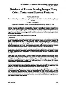
(a)Airplane

(b) Buildings

(d) Parkinglot (e) Tenniscourt Figure 3. Examples of Remote Sensing Images

(c)Overpass


∆𝑖𝑖+1 = 0.9∆𝑖𝑖 + 𝜂𝜂

469

𝜕𝜕𝜕𝜕

(16)

𝜕𝜕𝑊𝑊𝑖𝑖𝑙𝑙

𝑙𝑙 𝑊𝑊𝑖𝑖+1 = 𝑊𝑊𝑖𝑖𝑙𝑙 + ∆𝑖𝑖+1

(17)

Where i is iterative index, l is the number of layer (𝑙𝑙 ∈ {1,2,3}), 𝜂𝜂 is step. The initialization of the filter weights of each layer will be given by means of 0, standard deviation of 0.001 and the Gauss distribution of deviation of 0. In this way, good weight variance and the model of superresolution reconstruction of remote sensing image can be trained through the whole deep convolutional neural network, which is called as SRCNN [16]. 5. Experiment results and analysis In this paper, the superresolution reconstruction algorithm based on the convolution neural network is specially designed for the remote sensing image. The algorithm is trained under the framework of Caffe, including five categories (overpass, buildings, parkinglot, tenniscourt, and airplane) as shown in Figure 3. Each category includes 50 images size of 256 * 256 for training with a total of iteration of the 1.5 million times and spends about 170 hours. In the training process, the total 250 remote sensing images are down-sampled to get low resolution images. Then, mapping relationships between low resolution images and high resolution images are obtained. At last, the superresolution reconstruction algorithm finds appropriate training parameters through iteration, and finally gets the model suitable for remote sensing image super-resolution reconstruction. This paper evaluates the advantages and disadvantages of the superresolution reconstruction algorithm based on the deep convolutional neural network from subjective and objective aspects. In the subjective evaluation, as shown in Figure 4 and Figure 5, the reconstruction effect of Buildings can be seen clearly. The algorithm proposed in this paper can keep the details information and the visual effect is better. In the objective evaluation, the peak to noise ratio (PSNR) and structural similarity (SSIM) are used to evaluate the quality of remote sensing image reconstruction. Table 1 gives the reconstruction performance of superresolution reconstructed results by different methods, including bicubic, Yang, Zeyde, GR, Anchored Neighborhood Regression (ANR), Neighbor Embedding with Least Square decomposition (NE+LS), Neighbor Embedding with Non-Negative Least Squares decomposition (NE+NNLS), Neighbor Embedding with Locally Linear Embedding (NE+LLE) and SRCNN. It can be seen that PSNR of the reconstructed by SRCNN has significantly been improved compared to other algorithms, especially for Overpass image. According to SSIM, the superresolution reconstruction algorithm based on the deep convolutional neural network is better than previous algorithms. Therefore, in this paper, the proposed algorithm cannot only satisfy the visual effects of the human eye in the visual system, but also improve the objective evaluation index.

Parameter

PSNR（dB）

SSIM

Table 1. Superresolution reconstructed images comparison by different methods NE+ Methods Bicubic Yang Zeyde GR ANR NE+LS NNLS Overpass 27.5 28.9 29.1 28.4 28.8 28.9 28.3 Building 21.6 22.9 22.9 22.5 22.8 22.7 22.6 Parkinglot 26.7 27.2 28.5 28.9 28.5 28.2 28.2 Tenniscount 25.4 26.2 26.3 26.1 26.3 26.2 26.0 Airplane 25.2 25.8 26.2 25.9 26.1 26.0 25.8 Overpass 0.85 0.87 0.89 0.87 0.88 0.89 0.88 Buildings 0.74 0.79 0.80 0.77 0.79 0.79 0.78 Parkinglot 0.86 0.88 0.89 0.89 0.90 0.89 0.88 Tinniscourt 0.70 0.74 0.75 0.74 0.75 0.74 0.74 Airplane 0.75 0.77 0.79 0.77 0.78 0.78 0.78

NE+ LLE 28.8 22.7 28.5 26.2 26.1 0.88 0.79 0.89 0.75 0.78

SRCNN 30.5 24.0 29.2 26.6 26.5 0.91 0.84 0.91 0.76 0.79

6. Conclusions In this paper, the deep convolutional neural network is introduced into superresolution reconstruction of remote sensing images. A series of remote sensing images are chosen as the training set, and the mode is trained which is suitable for remote sensing image superresolution reconstruction. The experiment shows that the method has a good effect on the super resolution reconstruction of remote sensing image. In the future, we need to further explore the new deep learning network structure to enhance superresolution reconstruction of remote sensing images algorithm.

470


(a)LR image

(d) Bicubic

(g) Zeyde

(b)HR image

(e) Yang

(h) GR

(j) NE+LS (k) NELLE Figure 4. Reconstruction Results of Parkinglot

(c)SRCNN

(f) NE+NNLS

(i) ANR


(a)LR imag

(b)HR image

(d) Bicubic

(e) Yang

(g) Zeyde

(h) GR

471

(c)SRCNN

(f) NE+NNLS

(i) ANR

(j) NE+LS (k) NELLE Figure 5. Reconstruction results of overpass

References 1. 2.

Z. Cui, H. Chang and S. Shan, “Deep Network Cascade for Image Super-resolution,” Computer Vision – ECCV 2014. Springer International Publishing, pp.49-64, 2014. C. Dong, L. C. Chen and K. He, “Image Super-Resolution Using Deep Convolutional Networks,” IEEE Transactions on

472


3. 4.

5.

6. 7. 8. 9. 10. 11. 12. 13. 14. 15. 16.

17. 18.

Pattern Analysis & Machine Intelligence, 38(2), pp.295-307, 2016. A. Devi, T. Geetha, Madhum and K. Lal Kishore. : “A Novel Super Resolution Algorithm based on Fuzzy Bicubic Interpolation Algorithm,” International Journal of Signal Processing, Image Processing and Pattern Recognition, 8(8), pp.283-298, 2015. A. Devi, T. Geetha, Madhum and K. Lal Kishore. : “An improved super resolution image reconstruction using SVD based fusion and blind deconvolution techniques.” International Journal of Signal Processing, Image Processing and Pattern Recognition, 7(1), pp.283-298, 2014. L. Liebel and M. Körner, “Single-Image Super Resolution for Multispectral Remote Sensing Data Using Convolutional Neural Networks,” ISPRS-International Archives of the Photogrammetry, Remote Sensing and Spatial Information Sciences, pp.883890, 2016. Q. Luo, X. Shao and L. Wang, “Super-resolution imaging in remote sensing,” Proceedings of SPIE - The International Society for Optical Engineering, 9501(1), pp.175–181, 2015. S. Liu, Y. Zhu and L. Xue, “Remote sensing image super-resolution method using sparse representation and classified texture patches,” Wuhan Daxue Xuebao, 40(5), pp.578-582, 2015. Tang and Ling, “Blind Super-Resolution Image Reconstruction Based on Weighted POCS,” International Journal of Multimedia & Ubiquitous Engineering, 11(5), pp.367-376, 2016. H. Tao, X. Tang and J. Liu, “Super-resolution remote sensing image processing algorithm based on wavelet transform and interpolation,” Proceedings of SPIE-The International Society for Optical Engineering, 4898, pp.259-263, 2002. R. Timofte, D. V. Smet and V. L. Gool, “A+: Adjusted Anchored Neighborhood Regression for Fast Super-Resolution,” Computer Vision -- ACCV 2014, pp.111-126, 2015. W. Wang, H. Li, X. Zhang: “Fusion Algorithm of Remote Sensing Images Based on Nonsubsampled Pyramid and Empirical Mode of Demoposition,” Journal of Harbin Engineering, 11, pp.1394-1398, 2012. W. Wu, X. Yang and K. Liu, “A new framework for remote sensing image super-resolution: Sparse representation-based method by processing dictionaries with multi-type features,” Journal of Systems Architecture, 64, pp.63-75, 2016. W. Wu, X. Lu, Yang and K. Liu, “A new framework for remote sensing image super-resolution: Sparse representation-based method by processing dictionaries with multi-type features,” Journal of Systems Architecture, 67, pp.105-117, 2016. Z. Wang, Y. Yang and Z. Wang, “Learning Super-Resolution Jointly from External and Internal Examples,” IEEE Transactions on Image Processing A Publication of the IEEE Signal Processing Society, 24(11), pp.4359-4371, 2015. C. J. Yang, J. Wright and T. Huang, “Image super-resolution via sparse representation,” IEEE Transaction on Image Processing. 19(11), pp.2861-2873, 2010. X. Yang, W. Wu and W. Chen, “Remote Sensing Image Super-resolution Using Dual-Dictionary Pairs Based on Sparse Presentation and Multiple Features,” Proceedings of International Conference on Internet Multimedia Computing and Service. ACM, pp.90-94, 2014. Y. Zhao, J. Yang, W. C. Chan, “Hyperspectral Imagery Super-Resolution by Spatial–Spectral Joint Nonlocal Similarity,” IEEE Journal of Selected Topics in Applied Earth Observations & Remote Sensing 7(6), pp.2671-2679, 2014. Y. Zhang, W. Wu, Y. Dai, “Remote Sensing Images Super-resolution Based on Sparse Dictionaries and Residual Dictionaries,” IEEE International Conference on Dependable, Autonomic and Secure Computing, pp.318-323, 2013.