International Archives of the Photogrammetry, Remote Sensing and Spatial Information Sciences, Volume XL-1/W3, 2013 SMPR 2013, 5 – 8 October 2013, Tehran, Iran
SUPERVISED CLASSIFICATION OF POLARIMETRIC SAR IMAGERY USING TEMPORAL AND CONTEXTUAL INFORMATION A.Dargahia,*, Y.Maghsoudib, A.A.Abkarb a
Faculty of Geodesy and Geomatics Engineering, K.N. Toosi University of Technology, Vali-Asr St., Mirdamad Crossing, P.O. Box 15875-4416, Tehran 19967-15433, Iran –
[email protected] b Faculty of Geodesy and Geomatics Engineering, K.N. Toosi University of Technology, Vali-Asr St., Mirdamad Crossing, P.O. Box 15875-4416, Tehran 19967-15433, Iran – (ymaghsoudi, abkar)@kntu.ac.ir
KEY WORDS: Synthetic Aperture Radar (SAR), Polarimetry, Markov Random Field (MRF), Contextual Classification, Statistical Modeling, Forest
ABSTRACT: Using the context as a source of ancillary information in classification process provides a powerful tool to obtain better class discrimination. Modelling context using Markov Random Fields (MRFs) and combining with Bayesian approach, a context-based supervised classification method is proposed. In this framework, to have a full use of the statistical a priori knowledge of the data, the spatial relation of the neighbouring pixels was used. The proposed context-based algorithm combines a Gaussian-based wishart distribution of PolSAR images with temporal and contextual information. This combinat ion was done through the Bayes decision theory: the class-conditional probability density function and the prior probability are modelled by the wishart distribution and the MRF model. Given the complexity and similarity of classes, in order to enhance the class separation, simultaneously two PolSAR images from two different seasons (leaf-on and leaf-off) were used. According to the achieved results, the maximum improvement in the overall accuracy of classification using WMRF (Combining Wishart and MRF) compared to the wishart classifier when the leafon image was used. The highest accuracy obtained was when using the combined datasets. In this case, the overall accuracy of the wishart and WMRF methods were 72.66% and 78.95% respectively.
1. INTRODUCTION Polarimetric SAR (PolSAR) imagery provides a unique allweather mapping capability for terrain categorization and groundcover classification. Classification is one of the most widely used algorithms for extracting information from remotely sensing images. In recent decades PolSAR images due to their rich information content from environment has become one of the most useful remote sensing data sources. In general, for the classification of polarimetric images, two sources of information are used; the scattering mechanism and the statistical distribution. The early and most important classification methods based on scattering mechanisms is proposed by Van Zyl and Cloude (Van Zyl 1989; Cloude and Pottier 1997) led to the introduction of a widely used unsupervised classification scheme. These methods has been developed and improved in future work (Lee, Grunes et al. 2004). Gaussian-based wishart distribution (Goodman 1963) is the best known statistical distribution of polarimetric images, and wishart classifier is also one of the basic methods to classify PolSAR images (Lee, Grunes et al. 1994). In some research, non-Gaussian distributions used to analyze the PolSAR images. For example, in order to analysis the PolSAR images, several types of non-Gaussian distribution were used (Lee, Schuler et al. 1994; Freitas, Frery et al. 2005; Doulgeris, Anfinsen et al. 2011). Methods mentioned above, only using the single-pixel polarimetric data in classification and segmentation. For instance, classification based on scattering measurements of individual pixel, result in the isolated pixels and heterogeneous classes. Using the contextual information in classification and segmentation process improved accuracy the results and homogenization of classes. Markov Random Fields (MRFs)
(Geman and Geman 1984) provide a useful tool for combining contextual information into the classification process. Some researchers, for the segmentation of PolSAR images, have used a combination of non-Gaussian distributions (like kwishart) and contextual information within an MRF framework (Akbari, Doulgeris et al. 2013). This paper addresses the supervised contextual classification method based on the modelling context using MRFs and combining with Bayesian approach. In this proposed context-based algorithm using Gaussian-based wishart distribution of PolSAR images. For modelling contextual information by MRFs, an isotropic model with a second-order neighbourhood system, and to find the maximum posterior probability (minimum energy function), Iterated Conditional Modes (ICM) method were used.
2. THEORETICAL FOUNDATION 2.1 Full Polarimetry In the monostatic polarimetric SAR, H or V transmitted polarization coupled with H or V received polarization, produce the full scattering matrix (Lee and Pottier 2009):
[
(1)
]
Where the matrix S is named as scattering matrix and the S ij are the so-called complex scattering coefficients or complex scattering amplitudes. under the assumption of scattering reciprocity (Nghiem, Yueh et al. 1992) the SH V and SVH elements of the scattering vector are equal, and the
This contribution has been peer-reviewed. The peer-review was conducted on the basis of the abstract.
107
International Archives of the Photogrammetry, Remote Sensing and Spatial Information Sciences, Volume XL-1/W3, 2013 SMPR 2013, 5 – 8 October 2013, Tehran, Iran
backscattering of a monostatic polarimetric SAR system is characterized by the complex scattering vector:
[
]
√
(2)
Where the superscript T denotes matrix transpose. Usually, radar speckle can be suppressed by averaging several looks to reduce the noise variance. This procedure is called multilook processing. multilooked polarimetric covariance matrix is as follow:
∑ ∈ {
(7)
)
}∈
Where, is the neighbourhood of the r∈S, and c2 is known as a pairwise cliques, and V2 is called the potential function with respect to pairwise cliques. According to the assumption of isotropy, there is a single MRF model parameter (β>0) which is known as the spatial interaction parameter of the pairwise cliques and the potential can therefore be simplified to (Li 2009):
(8)
{
(3)
∑
(
3. METHOD AND DATASETS Where, n is the number of looks and superscript H means complex conjugate transpose and the vector is the ith 1-look sample. It follows that if n ≥ q (dimensions of vector ) and the in (3) are independent, then the scaled covariance matrix, defined as A=nZ, follows the non-singular complex Wishart distribution:
3.1 Method If event is the ith pattern vector and wj is information class j then, according to Equation (9), the probability that belongs to class wj is given by:
(4)
( |
(
)
|
)
(9)
Since, in general, P( ) is set to be uniformly distributed (i.e., the probability of occurrence is the same for all pixel features), Equation (9) can be rewritten as:
Where, C is class covariance matrix and,
(5) (
|
)
(
|
)
(10)
Where, Γ(·) is the gamma function. 2.2 Markov Random Field model Let a set of random variables d= {d1, d2, …, dm} be defined on the set S containing m number of sites in which each random variable yi (1≤ i≤ m) takes a label from label set L. The family d is called a random field. Given the definition of a random field specified above, we define the configuration w for the set S as w= {d1= w1, d2= w2,…, dm= wm}, where wr∈L (1 ≤ r ≤ m). A random field, with respect to a neighbourhood system is a MRF if the Markovian property holds for each site S. According to the Hammersley-Clifford theorem (Besag 1974), the joint probability distribution of a MRF is a Gibbs distribution. Therefore, the PDF of has the form (Li 2009; Tso and Mather 2009):
[
]
(6)
Where, N is a constant termed temperature (which should be assumed to take the value 1), and is the normalizing constant, and U(w) is called an energy function is as follows:
One can thus allocate pixel i to the class k, which has the largest ( | ) in Equation (10). The value of the term classification criterion can be expressed as { (
̂
|
)
}
(11)
The criterion shown in Equation (11) is called the Maximum A Posteriori (MAP) solution, which maximizes the product of conditional probability and prior probability. One of the methods for the estimate MAP is Iterated Conditional Modes (ICM) algorithm (Besag 1986). Based on ICM algorithm assumptions, The MAP estimation is now transformed to maximize Equation (12), which can be done by maximizing ( | ) on each pixel i locally, and Nr are neighbourhood pixels of jth pixel.
(
|
)
∏ (
|
(12)
)
| ) is Where, for polarimetric covariance matrix, ( obtained using (4), and base on MRFs can be described as:
This contribution has been peer-reviewed. The peer-review was conducted on the basis of the abstract.
108
International Archives of the Photogrammetry, Remote Sensing and Spatial Information Sciences, Volume XL-1/W3, 2013 SMPR 2013, 5 – 8 October 2013, Tehran, Iran
( |
)
{ ∑
} {
(13) }
{
4.1 Pre-processing
}
∑
{
}
Where, t is total number of classes, wj label of central pixel in neighbourhood system. In Equation (13), ( ) is the number of pixels with class labels equal to wj in Nr. Substitution, the Equation (4) and (13) in Equation (12): ( |
)
(14) (
)
{ ∑
4. RESULTS AND DISCUSSION
} {
}
Tow pre-processing steps were taken before using the SAR data for classification: speckle filtering and geometric correction. Speckle complicates image interpretation and analysis as well as decreases the effectiveness of image classification. In this study, we used the 5×5 window for speckle filtering. The second step of pre-processing was geometric correction. For the geometric correction of Polarimetric covariance matrix, MapReady software was used (Gens and Logan 2003). Pixels size in the output image after geometric correction, proportional to spatial resolution of RADARSAT-2 image in FQ9 mode, was chosen equal to 10 meter. The total root mean squared error (RMSE) of the geocoding using a set of 26 check points was 1.2 pixels. 4.2 Classification Results
Where, is the average covariance matrix of class wj, and n is number of look (Equivalent Number of Looks (ENL)) in multilook processing, and β=1.4 is adopted based on trial and error. The discriminant function of the popular Wishart classifier (Lee, Grunes et al. 1994) avoids dependency upon the ENL (n) by the restrictive assumption of equiprobable classes. For nontrivial choices of prior probability, Bayesian classifiers (like Equation (14)) based on the Wishart distribution or more sophisticated data models require an estimate of the ENL. Therefore, we need to calculate ENL. In this work, we used the method proposed by (Anfinsen, Doulgeris et al. 2009) to calculate the ENL. 3.2 Study Area and Datasets The study site selected is located near Chalk River, Ontario (45 ◦ 57’ N, 77◦ 34’ W) and includes the Petawawa Research Forest (PRF) and Canadian Forces Base (CFB) Petawawa. Reference data were collected from a circa 2002 forest inventory map, aerial photographic interpretation, Landsat ETM+ images and field visits. A total of five classes were considered in this study including red oak (OR), white pine (PW), black spruce (SB), ground vegetation (GV) and water (WA). A set of images covering the PRF site were acquired by Radarsat-2 with the fine quad-polarized (FQ) imaging mode. We collected images at two epochs for this study: a leaf-on image was collected on August 4, 2009; and a leaf-off image was collected on November 8, 2009. An image subset, which covers a forest area of approximately 15×16 km2, was selected for testing the classification algorithms. The detailed explanation of these datasets can be found in (Maghsoudi, Collins et al. 2012).
.CLASS NAMES
The results shown in three different modes, including leaf-on, leaf-off and a combined leaf-on&off (temporal) images, with two contextual and non-contextual classification methods were implemented. In the contextual classification (WMRF), the polarimetric information is contained in the wishart distribution and the context information is obtained through the use of MRF, whereas the non-contextual classification only employs the wishart distribution to as the statistical distribution of the polarimetric SAR data. In Table 1, reports the classification accuracy for the three dataset. As can be inferred, the classification results have been improved when using the proposed context-based algorithm. This improvement was observed in all the employed images. The highest accuracy was obtained when using the WMRF method over the combined leaf-on&off image. In this case, the overall accuracy of the wishart and WMRF methods were 72.66% and 78.95% respectively. Fig. 1 compares the classified images in the contextual and non-contextual cases for the leaf-on, leaf-off and leaf-on&off images. As can be seen, using the contextual methods a more homogenous classification is obtained.
5. CONCLUSIONS In this research, to classify PolSAR image, contextual information was used. Modeling contextual information and combining it with the statistical distribution of PolSAR images, we use MRF framework. We tested the proposed algorithm over three different modes of datasets and showed the classification accuracies before and after using contextual information.
Leaf-on
Leaf-off
Leaf-on&0ff
Wishart
WMRF
Wishart
WMRF
Wishart
WMRF
Red oak (OR)
43.26
46.58
39.31
44.55
59.40
69.73
White pine (PW)
41.66
52.78
39.37
45.14
49.57
57.87
Black spruce (SB)
39.66
50.40
40.34
53.49
50.74
65.37
Ground vegetation (GV)
69.95
75.65
84.69
91.02
84.23
87.85
100
100
98.30
98.36
99.88
99.94
63.15
70.52
65.46
70.84
72.66
78.95
Water (W) Overall Accuracy (OA)%
Table 1. Classification Accuracies (%) in Different Classes Using the Leaf-on, Leaf-off and Leaf-on&off Dataset
This contribution has been peer-reviewed. The peer-review was conducted on the basis of the abstract.
109
International Archives of the Photogrammetry, Remote Sensing and Spatial Information Sciences, Volume XL-1/W3, 2013 SMPR 2013, 5 – 8 October 2013, Tehran, Iran
a
b
d OR
PW
e SB
c
f GV
WA
Fig. 1. The Classified Images Using the Wishart Algorithm on Leaf-on (a), Wishart Algorithm on Leaf-off (b), Wishart Algorithm on Leaf-on&off (c), WMRF Algorithm on Leaf-on (d), WMRF Algorithm on Leaf-off (e), WMRF Algorithm Leaf-on&off (f).
6. REFERENCES Akbari, V., A. P. Doulgeris, et al. (2013). "A Textural– Contextual Model for Unsupervised Segmentation of Multipolarization Synthetic Aperture Radar Images." Anfinsen, S. N., A. P. Doulgeris, et al. (2009). "Estimation of the equivalent number of looks in polarimetric synthetic aperture radar imagery." Geoscience and Remote Sensing, IEEE Transactions on 47(11): 3795-3809. Besag, J. (1974). "Spatial interaction and the statistical analysis of lattice systems." Journal of the Royal Statistical Society. Series B (Methodological): 192236. Besag, J. (1986). "On the statistical analysis of dirty pictures." Journal of the Royal Statistical Society. Series B (Methodological): 259-302. Cloude, S. R. and E. Pottier (1997). "An entropy based classification scheme for land applications of polarimetric SAR." Geoscience and Remote Sensing, IEEE Transactions on 35(1): 68-78. Doulgeris, A. P., S. N. Anfinsen, et al. (2011). "Automated non-Gaussian clustering of polarimetric synthetic aperture radar images." Geoscience and Remote Sensing, IEEE Transactions on 49(10): 3665-3676. Freitas, C. C., A. C. Frery, et al. (2005). "The polarimetric " Environmetrics 16(1): 13-31. Geman, S. and D. Geman (1984). "Stochastic relaxation, Gibbs distributions, and the Bayesian restoration of images." Pattern Analysis and Machine Intelligence, IEEE Transactions on(6): 721-741. Gens, R. and T. Logan (2003). Alaska Satellite Facility software tools, Geophysical Institute, University of Alaska, Fairbanks, Alaska.
Goodman, N. (1963). "Statistical analysis based on a certain multivariate complex Gaussian distribution (an introduction)." Annals of Mathematical Statistics: 152-177. Lee, J., D. Schuler, et al. (1994). K-distribution for multilook processed polarimetric SAR imagery. Geoscience and Remote Sensing Symposium, 1994. IGARSS'94. Surface and Atmospheric Remote Sensing: Technologies, Data Analysis and Interpretation., International, IEEE. Lee, J. S., M. R. Grunes, et al. (1994). "Classification of multi-look polarimetric SAR imagery based on complex Wishart distribution." International Journal of Remote Sensing 15(11): 2299-2311. Lee, J. S., M. R. Grunes, et al. (2004). "Unsupervised terrain classification preserving polarimetric scattering characteristics." Geoscience and Remote Sensing, IEEE Transactions on 42(4): 722-731. Lee, J. S. and E. Pottier (2009). Polarimetric radar imaging: from basics to applications, CRC. Li, S. Z. (2009). Markov random field modeling in image analysis, Springer. Maghsoudi, Y., M. Collins, et al. (2012). "Polarimetric classification of Boreal forest using nonparametric feature selection and multiple classifiers." International Journal of Applied Earth Observation and Geoinformation 19: 139-150. Nghiem, S., S. Yueh, et al. (1992). "Symmetry properties in polarimetric remote sensing." Radio Science 27(5): 693-711. Tso, B. and P. Mather (2009). Classification methods for remotely sensed data, CRC. Van Zyl, J. J. (1989). "Unsupervised classification of scattering behavior using radar polarimetry data." Geoscience and Remote Sensing, IEEE Transactions on 27(1): 36-45.
This contribution has been peer-reviewed. The peer-review was conducted on the basis of the abstract.
110