structure, l2âstability, mean-value theorem, perceptron learning, positive realness, robust algorithm, small gain theorem. I. INTRODUCTION. APPLICATIONS of ...
612
IEEE TRANSACTIONS ON NEURAL NETWORKS, VOL. 8, NO. 3, MAY 1997
Supervised Learning of Perceptron and Output Feedback Dynamic Networks: A Feedback Analysis via the Small Gain Theorem Markus Rupp and Ali H. Sayed, Member, IEEE
Abstract—This paper provides a time-domain feedback analysis of the perceptron learning algorithm and of training schemes for dynamic networks with output feedback. It studies the robustness performance of the algorithms in the presence of uncertainties that might be due to noisy perturbations in the reference signals or to modeling mismatch. In particular, bounds are established on the step-size parameters in order to guarantee that the resulting algorithms will behave as robust filters. The paper also establishes that an intrinsic feedback structure can be associated with the training schemes. The feedback configuration is motivated via energy arguments and is shown to consist of two major blocks: a time-variant lossless (i.e., energy preserving) feedforward path and a time-variant feedback path. The stability of the feedback structure is then analyzed via the small gain theorem and choices for the step-size parameter in order to guarantee faster convergence are deduced by appealing to the mean-value theorem. Simulation results are included to demonstrate the findings. Index Terms—Convergence speed, dynamic networks, feedback structure, l2 –stability, mean-value theorem, perceptron learning, positive realness, robust algorithm, small gain theorem.
I. INTRODUCTION
A
PPLICATIONS of neural networks span a variety of areas in pattern recognition, filtering, and control. When supervised learning is employed, a training phase is always necessary. During this phase, a recursive update procedure is used to estimate the weight vector of the linear combiner that “best” fits the given data [1]–[3]. The recursive procedure often requires that a suitable adaptation gain (or step-size parameter) be chosen and, in most cases, heuristics and trial-and-error experiences are used to select a suitable step-size value for the training period. The “common” practice has been to choose small adaptation gains. But the smaller the adaptation gain the slower the convergence speed. In several cases, especially in large-scale applications with many weights and many training patterns, this may require a considerable amount of time and machine power.
Manuscript received July 10, 1995; revised June 19, 1996 and December 20, 1996. This work was supported by the National Science Foundation under Award MIP-9409319 and a scholarship from DAAD (German Academic Exchange Service) as well as the scientifical division of NATO. M. Rupp is with the Wireless Technology Research Dept., Lucent Technologies, Holmdel, NJ 07733–0400 USA. A. H. Sayed is with the Department of Electrical Engineering, University of California, Los Angeles, CA 90095 USA. Publisher Item Identifier S 1045-9227(97)02757-4.
In recent work on the robustness analysis of adaptive schemes [4]–[6], the authors have addressed the following two issues. 1) We have shown how to select the adaptation gain in order to guarantee a robust behavior in the presence of noise and modeling uncertainties (i.e., in order to guarantee a consistent performance in the sense that “small disturbances” would lead to “small estimation errors”). 2) We have also shown how to select the adaptation gain in order to guarantee faster convergence speeds. The formulation in [4]–[6] highlights an intrinsic feedback structure for most adaptive schemes and it relies on tools from system theory, control, and signal processing such as: state-space descriptions, feedback analysis and the small gain theorem, H -design, and transmission lines and lossless systems. In this paper we address the implications of these results to the training of perceptrons and recurrent neural networks. We start by considering the so-called perceptron learning algorithm (PLA, for short), which involves a nonlinear functional in the update equation due to the presence of an activation function (usually a sigmoid function). We show how to extend the feedback arguments of [4] and [5] in order to handle the presence of the nonlinearity and, as a fallout, we suggest several choices for the step-size parameter in order to guarantee faster convergence and robust performance. We also establish the existence of a feedback structure that can be associated with the PLA. The feedback configuration is motivated via energy arguments and is shown to consist of two major blocks: a time-variant lossless (i.e., energy preserving) feedforward path and a time-variant feedback path. The analysis applies to both cases when the feedback path is static or dynamic (which occurs in the case of recurrent networks), and it provides physical insights into the energy propagation through the feedback system. This enables us to suggest modifications to the training algorithm, in terms of selections of the adaptation gain, in order to accelerate the convergence speed during the training phase. In the later sections of the paper, we extend the time-domain feedback analysis of the PLA to dynamic neural networks (also recurrent neural networks or RNN’s) with output feedback [7], [8], and provide a study of the robustness performance of the
1045–9227/97$10.00 1997 IEEE
RUPP AND SAYED: SUPERVISED LEARNING OF PERCEPTRON
613
A. The Perceptron Learning Algorithm (PLA) with the correConsider a collection of input vectors sponding correct (or desired) output values . The are assumed to belong to the range of the activation function , i.e., there exists an unknown column vector such that for some
Fig. 1. The perceptron structure.
training phase in the presence of uncertainties. In this context, certain positive-realness conditions arise in much the same way as in the study of IIR adaptive filters and identification schemes [9]–[11]. Here, however, as indicated in the remark after inequality (40), a less restrictive condition is tolerable in view of the presence of the nonlinear activation function. A. Notation Small boldface letters are used to denote vectors (e.g., ), the letter “ ” to denote transposition, and to denote the Euclidean norm of a vector . Also, subscripts are used for time-indexing of vector quantities (e.g., ) and parenthesis for time-indexing of scalar quantities (e.g., ). All vectors are column vectors except for the row vectors .
(2)
This is in agreement with the models used in [13] and [14]. In supervised learning, the perceptron is presented with the given input-output data , and the objective is to estimate the unknown weight vector . The PLA computes recursive estimates of as follows. It starts with an arbitrary initial guess and applies the update rule (3) is the sigmoid activation function or, more generwhere ally, any monotonically increasing function. For generality, we consider in this paper the possibility of noisy perturbations in the reference signal. These can be due to model mismatching or to measurement noise.1 We denote the perturbed references by (which are now the given data instead of ), say (4) denotes the noise term. Correspondingly, we study where the following general form of recursion (3):
II. THE PERCEPTRON Consider two sets, and , of -dimensional real-valued row vectors that are characterized by either property or property , say has property has property If the two sets are linearly separable, then a classification scheme that can be used to decide whether a given vector belongs to one class or the other is to employ a perceptron device [1]–[3]. The perceptron consists of a linear combiner, whose column weight vector we denote by , followed by a nonlinearity (also known as an activation function), as depicted in Fig. 1. The value assumed by can be interpreted as the likelihood that the input vector belongs to one class or another. A common choice for is to employ the sigmoid function (1) This is a function that varies monotonically from to for , and its transition region around is more or less steep depending on whether the parameter is large or small. In particular, for , the sigmoid function collapses to the hard-limiting function if if
(5) replaces and where we have allowed for a where time-variant step-size parameter . We shall also, and without loss of generality, assume that the are nonzero. For a nonzero step-size , a zero simply corresponds to a nonactive update step since it keeps the weight estimate unaltered, i.e., . B. Error Measures The following error quantities are useful for our later analysis: denotes the difference between the true weight and its estimate , denotes the a priori estimation error, , and denotes the a posteriori estimation error, It follows from (5) that the weight-error vector satisfies the recursion: (6) C. Robustness Issues In the sequel we focus on model (4) and study the robustness behavior of the update recursion (5). Intuitively, a robust algorithm is one for which the estimation errors are consistent with the disturbances in the sense that “small” disturbances would lead to “small” estimation errors, no matter what the disturbances are! This is not generally true for any adaptive
1
1 Assume for example that the reference system employs f (z ) while the trained perceptron employs f (z ) with = 4. The differences, which occur mainly around z = 0, can be described by an additive noise term.
614
IEEE TRANSACTIONS ON NEURAL NETWORKS, VOL. 8, NO. 3, MAY 1997
filter: the estimation errors can still be large even in the presence of small disturbances (see, e.g., [12]). While a more precise mathematical formulation is provided in the sections to follow, we stress here that the motivation for our analysis is twofold. 1) To provide conditions on the adaptation gain (or stepsize parameter) in order to guarantee a robust behavior during the training phase. By this we mean a training algorithm that results in “small” errors if the disturbances are “small.” It turns out that such a desirable performance is not guaranteed for any choice of the step-size. 2) To suggest choices for the step-size parameter that would result in faster convergence speeds. The robustness issue is addressed here in a purely deterministic framework and without assuming prior knowledge of noise statistics. This is especially useful in situations where prior statistical information is missing since a robust design would guarantee a desired level of robustness independent of the noise statistics. In loose terms, robustness would imply that the ratio of an estimation error energy to the noise or disturbance energy will be guaranteed to be upper bounded by a positive constant, say the constant one estimation error energy disturbance energy
(7)
From a practical point of view, a relation of the form (7) is desirable since it guarantees that the resulting estimation error energy will be upper bounded by the disturbance energy, no matter what the nature and the statistics of the disturbances are. One of the contributions of this work is to show how to select the adaptation gains in (5) in order to guarantee 1) a robust behavior and 2) faster convergence. This is addressed in the next sections. III. A CONTRACTIVE MAPPING
If we now compute the squared norm (i.e., energies) of both sides of (9), we conclude that the following equality always holds:
This equality allows us to conclude that the following energy bounds are always satisfied, where we have introduced the parameter . Lemma 1: Consider the perceptron learning recursion (3)–(4). It always holds, at each time instant , that for if for where is the modified disturbance given by (8). The first two inequalities in the statement of the lemma establish that if the adaptation gain is chosen such that , then the mapping from the signals to the signals is contractive. [A linear map that takes to , say , is said to be contractive if for all we have That is, the output energy does not exceed the input energy]. Therefore, we see that the first two cases in the lemma establish a local error-energy bound (or passivity relation) that highlights a robustness property of recursion (5): They state that no matter what the value of the noise component is, and no matter how far the estimate is from the true vector , the sum of energies , will always be smaller than or equal to the sum of energies . Moreover, since this contractivity property holds for each time instant , it should also hold globally over an interval of time. Indeed, assuming over , it follows from Lemma 1 that
We first establish a passivity relation that shows how the sum of the Euclidean norms of the weight-error vector and the a priori estimation error at time
compares with the sum of the Euclidean norms of the weighterror vector at time and a disturbance term that is defined in (8) further ahead
We may remark that other similar local and global passivity relations can be established by using a posteriori (rather than a priori) estimation errors [6]. But we shall forgo the details here and focus instead on a time-domain and feedback analysis of the PLA. IV. A TIME-DOMAIN FEEDBACK-ANALYSIS
The significance (and implications) of the relation to be established here will become clear as we progress in our discussions. We denote the difference in (6) by and note that it is equal to , where the modified disturbance is defined by (8)
The bounds of Lemma 1 can be described in an alternative form that leads to an interesting feedback structure. For this purpose, we first note that it can also be shown that the update equation (5) can be written in the form (cf. the analysis in [4]) (10) where we have used the fact that
This allows us to rewrite (6) as (11) (9)
RUPP AND SAYED: SUPERVISED LEARNING OF PERCEPTRON
615
V.
-STABILITY
AND THE
SMALL GAIN THEOREM
Define
That is, is the maximum absolute value of the gain of the feedback loop over . It can be easily shown that if (see, e.g., [4]) then the following two relations hold: Fig. 2. A time-variant lossless mapping with gain feedback for the perceptron learning algorithm.
Consequently (14)
(12) Relation (12) has the same form as the update (9), except for a different disturbance ( is now replaced by ) and for a step-size that is equal to itself. Hence, the same arguments that led to Lemma 1 would imply that the following equality holds for all possible choices of :
and
(13) from the signals This establishes a lossless mapping to the signals . If we further apply the mean-value theorem to the activation function , we can write
for some point along the segment connecting . Therefore, (11) leads to
and
Combining with (13), this relation shows that the overall mapping from the original (weighted) disturbances to the resulting a priori (weighted) estimation errors can be expressed in terms of a feedback structure, as shown in Fig. 2. The stability of such feedback structures can be studied via tools that are by now standard in system theory (e.g., the small gain theorem [15], [16]). This is pursued in the next section where we derive conditions on the step-size parameters and on the activation function in order to guarantee a robust training algorithm, as well as faster convergence speeds. This will be achieved by establishing conditions under which the feedback configuration of Fig. 2 is -stable in the sense that it should map a finite-energy input noise sequence (which includes the noiseless case as a special case) to a finite-energy a priori error sequence .
(15) Expression (14) compares the energies of a priori estimation errors and the disturbances (but now normalized by rather than ). In particular, it establishes that the map from to is -stable (it maps a finite energy sequence to another finite energy sequence). The condition is a manifestation of the socalled small gain theorem in system analysis [15], [16]. In simple terms, the theorem states that the -stability of a feedback configuration (that includes Fig. 2 as a special case) requires that the product of the norms of the feedforward and the feedback maps be strictly bounded by one. Here, the feedforward map has ( -induced) norm equal to one (since it is lossless) while the -induced norm of the feedback map is . Hence, the condition guarantees an overall contractive map. Note also that for to hold, we need to choose such that, for all the step-size (16) A. On Convergence and Energy Propagation The flow of energy through the feedback connection of Fig. 2 provides further insights into the convergence speed of the training algorithm. For this purpose, let us ignore the measurement noise and assume that we have noiseless measurements . It is known in the stochastic setting that for Gaussian processes [18], as well as for spherically invariant random processes [19], the maximal speed of convergence for a gradient algorithm (where ) is obtained for , i.e., for the so-called projection LMS
616
IEEE TRANSACTIONS ON NEURAL NETWORKS, VOL. 8, NO. 3, MAY 1997
Fig. 3. Learning curves for perceptron learning algorithm with
=
0:4 and � = 0:6; 1; 2; 2:8.
algorithm. We now argue that this conclusion is consistent with the feedback configuration of Fig. 2. If is such that , then the feedback loop is disconnected. This means that there is no energy flowing back into the lower input of the lossless section from its lower output . The losslessness of the feedforward path then implies that (17) the energy of where we are denoting by and by the energy of . But what if ? In this case the feedback path is active and the convergence speed will be affected. Indeed, we now have
(18) . It is easy to where we have defined the coefficient verify that as long as is chosen to satisfy (16) with , we obtain . That is, is strictly less than one and the rate of decrease in the energy of is lowered. VI. OPTIMAL CHOICES
OF
STEP SIZES
The above energy arguments suggest that faster convergence occurs when is chosen such that (which is the middle point of the interval suggested by (16)). But is still unknown and we therefore need to come up with suitable approximations. The first (but not the most suitable) choice that comes to mind is to assume an upper bound on , say for all Then condition (16) can be replaced by the conservative requirement (19)
For a large bound , this condition can lead to small stepsizes and, hence, to slow convergence. For the commonly used activation functions, the maximum value of the derivative occurs at the origin. For example, for the sigmoid function we obtain . We can therefore take and choose the step-size parameter according to This is the same bound suggested in [14]. However, the result in [14] was derived under the restrictive assumption that the regression vectors do not change over time, i.e., for all . Our result thus extends the bound to the general scenario of time-variant regression vectors. For improved convergence one might then be tempted to employ However, this value is very conservative and usually leads to unsatisfactory results, as the simulations further ahead demonstrate. For this reason, we take here an alternative route that avoids upper-bounding the derivative of the activation function. Instead, we provide good estimates for the instantaneous derivatives . To begin with, recall that is defined by , where . and are not available since itself Unfortunately, is not known. But one possibility to proceed here is to employ as an estimate for since This is especially useful if the reference sequence is noise-free or if the noise itself is sufficiently small. Now, with a “known” , it becomes possible to solve for . This motivates us to suggest the following expression for the optimal step-size parameter (we refer to this construction as method A) (20) is used as a threshold value in order to prevent where large step-sizes. For the sigmoid function in (1) we have which requires the evaluation of a logarithm at each step. In the case of a symmetric , the sigmoid function, say calculation of an inverse tangent is required since .
RUPP AND SAYED: SUPERVISED LEARNING OF PERCEPTRON
617
An alternative procedure is to approximate by the average of (or ) and . This is a convenient approximation in light of the “piecewise-linear” form of the activation function. We thus write (21) . The where, for the sigmoid function, positive number is, similar to in method A, introduced in order to avoid large step-sizes. This approximation is however inconvenient in the cases when happens to be close to zero, while and are reasonably far apart. To avoid a poor approximation in these cases, we may modify the above construction as follows: for improved convergence (i.e., with a disconnected feedback loop) we set (22) if
or (23)
otherwise. We refer to this construction as method B. Condition (23) corresponds to the sigmoid function in (1). For a symmetrical function a similar expression can be obtained. A third, and perhaps simpler method, is to first estimate by the average of and , i.e., , and then set . This leads to method C, with the choice (24) Before extending the earlier results to dynamic networks, we present some simulations that support our conclusions. VII. SIMULATION RESULTS
FOR
PLA
In all experiments, we have chosen a bipolar white random sequence with variance one as the input signal. The weights to be identified were . The first coefficient was used for the offset term while the other eight were driven by a bipolar input pattern. A neuron with these weights can be interpreted as one that finds the patterns with more than three . The values of the inner signal are from the set . Since the 256 different input patterns consisted of the bipolar values , we had and at every time instant . We have chosen the sigmoid function (1) with . We provide plots of learning curves, given in terms of the relative system mismatch defined as . The curves are averaged over 50 Monte Carlo runs in order to approximate . Not depicted here are -curves. Their behavior is very much like the system mismatch curves, however, in order to obtain smooth curves they require more averaging.
The first simulation is for , for which the sigmoid function operates in an almost linear range. The resulting learning curves are depicted in Fig. 3. As expected from (19), and since the sigmoid function operates essentially in the linear region, the fastest convergence speed occurs for , while instability occurs for values . The next simulation shows learning curves for (see Fig. 4). With fixed step-sizes the fastest convergence was , while for the algorithm was found at already unstable. The bound (19) for which the largest possible step-size is given by is now too conservative and the proposed modifications (A), (B) and (C) lead to much faster convergence. For all methods, the step-size was chosen to be optimal (with and ). Since method (C) always showed the same behavior as (B) it is not depicted here. As the figure demonstrates, the first choice leads to excellent convergence, however, at the expense of calculating a logarithm at every time instant. The second choice, although not as perfect as the first one, still shows considerable improvement over the constant step-size choice. For the third simulation . According to (19), convergence is expected for . As Fig. 5 shows, for smaller than this bound convergence occurs. However, this bound is rather conservative and fastest convergence occurs for larger step-size values, viz., . A learning curve for still shows convergence but with some stopping effect. It seems noteworthy that even very large step-sizes can still lead to convergence, although the parameter estimates seem to diverge. This effect was not observed for small and seems to arise from the fact that the system behaves highly nonlinearly. This effect could also be observed for , where it was even stronger. Method (B), with the optimal choice for the step-size, was applied again and showed much faster convergence than any other choice of a constant step-size. Instability occurred for approximately . VIII. DYNAMIC NEURAL NETWORKS A. Vector Notation We show in the following sections how to extend the analysis to the recurrent neural network (RNN) case, for which we have selected Narendra and Parthasarathy’s network [7] since it is very suitable for the feedback analysis of the earlier sections. But first we introduce, for convenience of exposition, the following vector and matrix notation. Define the column vectors: (25) (26) and the diagonal matrices (27) (28) (29)
618
Fig. 4. Learning curves for perceptron learning algorithm with
IEEE TRANSACTIONS ON NEURAL NETWORKS, VOL. 8, NO. 3, MAY 1997
= 2 and � = 0:3; 0:6; 1 and �opt for methods (A) and (B).
Fig. 5. Learning curves for perceptron learning algorithm with = 4 and � = 0:1; 0:2; 0:4; 0:8 and �opt from method (B).
We write with a vector argument to indicate the dependence on the set . It is easy to see that, due to the diagonal structure of , and , the two-induced norms of the matrices and are equal to and , respectively. B. Narendra and Parthasarathy’s Recurrent Network Narendra and Parthasarathy’s recurrent network is a dynamic network whose current output is also a function of earlier output values, in much the same way as the output of an IIR filter is dependent on the previous outputs [2]. Fig. 6 depicts a block diagram of a recurrent structure suggested by Narendra and Parthasarathy [2], [7], [8]. The network consists of two linear combiners with weight vectors and . The upper combiner receives an external and evaluates the inner product . The row input vector lower combiner receives the state vector of an FIR filter and computes its inner product with . The FIR filter is fed with
Fig. 6. Narendra and Parthasarathy’s dynamic network.
the output given by
of the network and, hence, its state vector is
where is the order of the filter . The weight vector of the network of Fig. 6 is defined by . The objective of a training phase is to provide
RUPP AND SAYED: SUPERVISED LEARNING OF PERCEPTRON
619
Fig. 7. Narendra and Parthasarathy’s algorithm as a time-variant lossless mapping with dynamic feedback.
the network with a collection of input–output data, in order to estimate the unknown vectors and . Here
,
A recursive gradient-type scheme that can be used for the training of such a network is the following. Let and denote estimates for and at time , respectively. Let also denote the corresponding output, viz., (30)
and, consequently, the update equation (31) leads to
Following the arguments of [4], we can therefore write: (34) where the modified noise sequence
is defined by
where
and . This recursion is of the same form as (10). It then follows in a similar way that: The estimates for and are recursively evaluated as follows: start with arbitrary initial conditions for and , say an initial weight vector , and use (31) This can be regarded as an immediate extension of a so-called Feintuch algorithm [17] in IIR modeling (where is linear) to the case of Fig. 6, which now includes a nonlinear . A discussion in the IIR case, with activation function linear , can be found in [20]. Define and . Then (32)
(33) stands for the linear operator , and are the coefficients of the FIR filter . By invoking the mean-value theorem we can write , or, equivalently, for some in the interval connecting and . This allows us to conclude from (33) that
where
(35) to which establishes that the map from , denoted by , is lossless, and that the to the overall mapping from the original disturbance can be expressed resulting a priori estimation error in terms of the feedback structure shown in Fig. 7. We remark that the notation
which appears in the feedback loop, should be interpreted as follows: we first divide by , followed by the filter , and then by a subsequent scaling by
.
The feedback loop now consists of a dynamic system. But we can still proceed to study the -stability of the overall configuration in much the same way as we did in the former section. For this purpose, we use the vector and matrix quantities introduced in (26)–(28) and define a vector , similar to , but with the entries instead of . from (29), and the lowerWe also use the diagonal matrix triangular matrix that describes the action of the FIR filter on a sequence at its input; this is a strictly lower-triangular
620
IEEE TRANSACTIONS ON NEURAL NETWORKS, VOL. 8, NO. 3, MAY 1997
This condition has an interesting connection with the linear filtering case. For Feintuch’s algorithm [17], the sign of is relevant to the stability of the algorithm. Here, the additional term can compensate for this effect and even negative values for are allowed (see the simulation examples). For a sigmoid function , we know that lies in the range . Therefore, in this case, a sufficient condition for (37) is given by the relation
Toeplitz matrix with band of width
.. .
..
.
..
.
..
.
It follows from (35) that we can write:
(41) If we now define IX. SIMULATION RESULTS FOR NARENDRA AND PARTHASARATHY’S NETWORK and impose the condition , we obtain that a single-neuron Narendra and Parthasarathy’s network will be -stable in the sense that the map from to satisfies
In the simulation that follows, a bipolar white random sequence with variance one has been used for the entries of the input vector . A plot of the learning curve is provided for the relative system mismatch defined as
(36) Moreover, the map from will also be -stable with
The curves are averaged over 50 Monte Carlo runs in order to approximate . Similar curves can be obtained if is used instead. For simulating the behavior of Narendra and Parthasarathy’s network, two different sets of values has been chosen with eight input weights, one offset, and two feedback weights
to
The robustness (or -stability) condition corresponds to requiring the feedback matrix to be contractive, i.e.,
and
(37) If we limit ourselves, for simplicity, to the case of constant step-sizes , then a sufficient condition for (37) is to require (38) Let
The first weight vector corresponds Re , while the second weight vector corresponds to Re . Fig. 8 shows the learning curves for and when the set was used. In order to provide a symmetrical feedback input the following sigmoid function was applied
Then a sufficient condition for (38) is to require
which in turn is satisfied if
If we have an a priori bound on
, say (39)
then a sufficient condition for (37) to be satisfied is to choose such that (40)
which has the same maximal derivative as the one defined in (1), i.e., . Since the filter inputs are { 1, 1} patterns and the output is also limited to [ 1,1] we can use and according to bound (40) the training phase converges if for in the case of . Fig. 8 depicts two learning curves for and for which we found fastest convergence. Instability occurred for which is in good agreement with (40). The second (non-SPR) filter showed very similar behavior. Because of the negative real part, the limit step-size is smaller. However, unstable behavior as in the Feintuch algorithm does not occur here. As a general rule of thumb one can say that the larger the , and thus the larger the influence of the nonlinearity, the smaller the step-size that is is required for stability.
RUPP AND SAYED: SUPERVISED LEARNING OF PERCEPTRON
Fig. 8. Learning curves for Narendra and Parthasarathy’s network (a) � � = 0:2; = 4, (e) method (C), = 4.
Also, for both filters, modifications as described before in Section VI can be suggested but they may or may not bring advantages in general. This is not surprising since we need to compensate the filtering effect of rather than only the effect of the derivative . However, for larger the effect of the derivative becomes stronger and may exceed the filter effect. This situation is of particular interest since the network with constant step-size has very poor convergence behavior [see Fig. 8 curves (c) and (d)]. Simulations were performed with the recurrent network by employing the optimal choices of Section VI. Fig. 8 curve (e) shows that method (C) [also (A) and (B)] can be used to accelerate the training phase considerably (for large ). X. CONCLUDING REMARKS We have provided a time-domain feedback analysis of training algorithms for perceptron and dynamic networks with output feedback. The derivation highlights a feedback structure in terms of a lossless feedforward path and either a memoryless or a dynamic feedback loop. The interconnection is amenable to analysis to standard tools in system theory, such as the small gain theorem, and indicates choices for the step-size parameters in order to guarantee both robustness and faster convergence speed. Several simulation examples are provided to support the theoretical findings. In the dynamic network case, certain positive-realness conditions arise in much the same way as in the study of IIR adaptive filters and identification schemes. Here, however, as indicated in the remark after (40), a less restrictive condition is tolerable in view of the presence of the nonlinear activation function. We may also mention that the analysis in this paper has focused on the case of single neurons (perceptrons and RNN’s) and has addressed questions related to the three issues of robustness, optimal step-sizes, and convergence. A local robustness analysis of the backpropagation algorithm that is employed in the training of multilayer perceptrons has been
621
=
0:5; = 0:4, (b) � = 1:1; = 0:4, (c) � = 0:1; = 4, (d)
provided in [21] by invoking results from H filtering. This analysis ties up nicely with the result in [12] that establishes that the instantaneous gradient-based (LMS) adaptive filter is a minimax filter; thus highlighting its robustness properties. A related discussion on these issues can also be found in the companion paper [5]. REFERENCES [1] S. Haykin, Neural Networks: A Comprehensive Foundation. New York: MacMillan, 1994. [2] D. R. Hush and B. G. Horne, “Progress in supervised neural networks,” IEEE Signal Processing Mag., vol. 10, no. 1, pp. 8–39, Jan. 1993. [3] R. P. Lippmann, “An introduction to computing with neural nets,” IEEE Acoust., Speech, Signal Processing Magazine, vol. 4, no. 2, pp. 4–22, Apr. 1987. [4] M. Rupp and A. H. Sayed, “A time-domain feedback analysis of filterederror adaptive gradient algorithms,” IEEE Trans. Signal Processing, vol. 44, pp. 1428–1439, June 1996. [5] A. H. Sayed and M. Rupp, “An l2 -stable feedback structure for nonlinear adaptive filtering and identification,” to appear in Automatica, 1997. , “Error-energy bounds for adaptive gradient algorithms,” IEEE [6] Trans. Signal Processing, vol. 44, pp. 1982–1989, Aug. 1996. [7] K. S. Narendra and K. Parthasarathy, “Identification and control of dynamical systems using neural networks,” IEEE Trans. Neural Networks, vol. 1, pp. 4–27, Mar. 1990. [8] , “Gradient methods for the optimization of dynamical systems containing neural networks,” IEEE Trans. Neural Networks, vol. 2, pp. 252–262, Mar. 1991. [9] L. Ljung and T. S¨oderstr¨om, Theory and Practice of Recursive Identification. Cambridge, MA: MIT Press, 1983. [10] I. D. Landau, “A feedback system approach to adaptive filtering,” IEEE Trans. Inform. Theory, vol. IT-30, Mar. 1984. [11] V. Solo and X. Kong. Adaptive Signal Processing Algorithms: Stability and Performance. Englewood Cliffs, NJ: Prentice-Hall, 1995. [12] B. Hassibi, A. H. Sayed, and T. Kailath, “H optimality of the LMS algorithm,” IEEE Trans. Signal Processing, vol. 44, pp. 267–280, Feb. 1996. [13] J. J. Shynk and N. J. Bershad, “On the system identification convergence model for perceptron learning algorithms,” in Proc. Asilomar Conf. Signals, Syst., Computers, Oct. 1994, pp. 879–886. [14] S. Hui and S.H. Zak, “The Widrow–Hoff algorithm for McCulloch–Pitts type neurons,” IEEE Trans. Neural Networks, vol. 5, pp. 924–929, Nov. 1994. [15] H. K. Khalil, Nonlinear Systems. New York: MacMillan, 1992. [16] M. Vidyasagar, Nonlinear Systems Analysis, 2nd ed. Englewood Cliffs, NJ: Prentice-Hall, 1993. [17] P. L. Feintuch, “An adaptive recursive LMS filter,” Proc. IEEE, vol. 64, no. 11, pp. 1622–1624, Nov. 1976.
1
622
IEEE TRANSACTIONS ON NEURAL NETWORKS, VOL. 8, NO. 3, MAY 1997
[18] N. J. Bershad, “Analysis of the normalized LMS algorithm with Gaussian inputs,” IEEE Trans. Acoust., Speech, Signal Processing, vol. ASSP34, pp. 793–806, Aug. 1986. [19] M. Rupp, “The behavior of LMS and NLMS algorithms in the presence of spherically invariant processes,” IEEE Trans. Signal Processing, vol. 41, pp. 1149–1160, Mar. 1993. [20] M. Rupp and A. H. Sayed, “On the stability and convergence of Feintuch’s algorithm for adaptive IIR filtering,” in Proc. IEEE Conf. ASSP, Detroit, MI, May 1995. [21] B. Hassibi, A. H. Sayed, and T. Kailath, “LMS and backpropagation are minimax filters,” in Neural Computation and Learning, V. Roychowdhury, K. Y. Siu, and A. Orlitsky, Eds. Boston, MA: Kluwer, 1994, ch. 12, pp. 425–447.
Markus Rupp received the Diploma in electrical engineering from FHS Saarbruecken, Germany, and Universit¨at Saarbruecken in 1984 and 1988, respectively. He received the Doctoral degree in 1993 summa cum laude at the TH Darmstadt in the field of acoustical echo cancellation. He received the DAAD Postdoctoral Fellowship and spent from November 1993 to September 1995 in the Department of Electrical and Computer Engineering of the University of California, Santa Barbara. From 1984 to 1988 he was a Lecturer in Digital Signal Processing and High Frequency Techniques at the FHS. Since October 1995 he has been with the Lucent Technologies, Wireless Technology Research Department, Homdel, NJ, where he is currently working on new adaptive equalization schemes. His interests include algorithms for speech applications, speech enhancement and recognition, echo compensation, adaptive filter theory, H -filtering, neural nets, classification algorithms, and signal detection. He has over 40 publications in the field of adaptive filters.
1
Ali H. Sayed (S’90–M’92) was born in S˜ao Paulo, Brazil. In 1981 he graduated in first place in the National Lebanese Baccalaureat, with the highest score in the history of the examination. In 1987 he received the bachelor’s degree in electrical engineering from the University of S˜ao Paulo, and was the first-place graduate of the School of Engineering. In 1989 he received the M.S. degree with distinction in electrical engineering from the University of S˜ao Paulo. In 1992 he received the Ph.D. degree in electrical engineering from Stanford University, Stanford, CA. From September 1992 to August 1993 he was a Research Associate with the Information Systems Laboratory at Stanford University, after which he joined, as an Assistant Professor, the Department of Electrical and Computer Engineering at the University of California, Santa Barbara. Since July 1996, he has been an Associate Professor in the Department of Electrical Engineering at UCLA. He has more than 70 publications. His research interests are in the areas of adaptive and statistical signal processing, linear and nonlinear filtering and estimation, interplays between signal processing and control methodologies, interpolation theory, and structured computations in systems and mathematics. Dr. Sayed is a member of SIAM and ILAS. He was awarded the Institute of Engineering Prize and the Conde Armando Alvares Penteado Prize, both in 1987 in Brazil. He was awarded an FAPESP fellowship for overseas studies in 1991 and his Ph.D. dissertation on structured algorithms in signal processing and mathematics received a special mention, among the top three Ph.D. dissertations written during the period from 1990 to 1993, for the Householder Prize in numerical algebra. He is a recipient of a 1994 NSF Research Initiation Award, and of the 1996 IEEE Donald G. Fink Prize Award. He is an Associate Editor of the IEEE TRANSACTIONS ON SIGNAL PROCESSING.