support vector classifier via mathematica - Völgyesi Lajos

SUPPORT VECTOR CLASSIFIER VIA MATHEMATICA B. PALÁNCZ1, L. VÖLGYESI2,3 1

Department of Photogrammetry and Geoinformatics 2 Department of Geodesy and Surveying Budapest University of Technology and Economics 3 Physical Geodesy and Geodynamic Research Group of the Hungarian Academy of Sciences H-1521 Budapest, Hungary e-mail: [email protected]

Abstract In this case study a Support Vector Classifier function has been developed in Mathematica. Starting with a brief summary of support vector classification method, the step by step implementation of the classification algorithm in Mathematica is presented and explained. To check our function, two test problems, learning a chess board and classification of two intertwined spirals are solved. In addition an application to filtering of airborne digital land image by pixel classification is demonstrated using a new SVM kernel family, the KMOD, a kernel with moderate decreasing. Keywords: software Mathematica, kernel methods, pixel classification, remote sensing.

Introduction Kernel Methods are relatively new family of algorithms that presents a series of useful features for pattern analysis in datasets. Kernel Methods combine the simplicity and computational efficiency of linear algorithms, such as the perception algorithm or ridge regression, with flexibility of nonlinear systems, such as for example neural networks, and rigour of statistical approaches such as regularization methods in multivariate statistics. As a result of the special way they represent functions, these algorithms typically reduce the learning step to convex optimization problem that can always be solved in polynomial time, avoiding the problem of local minima typical of neural networks, decision trees and other nonlinear approaches [1]. 1 Support Vector Classification 1.1 Binary classification In case of binary classification, we try to estimate a real-valued function f: X ⊆ R n → R using training data, that is n - dimensional patterns xi and class labels yi ∈ {−1, 1} (( x1 , y1 ), ..., ( xm , ym )) ∈ R n × {−1, 1}

such that f will correctly classify new examples (x, y) − that is, f(x) = y for examples (x, y), which were generated from the same underlying probability distribution P(x,y) as the training data. If we put no restriction on the class of functions that we choose

our estimate f from, however, even a function that does well on the training data − for example by satisfying f ( xi ) = yi for i = 1...m − need not generalize well to unseen examples. Suppose we know nothing additional about f (for example about its smoothness), then the values on the training patterns carry no information whatsoever about values on novel patterns. Hence learning is impossible, and minimizing the training error does not imply a small expected test error. Statistical learning theory, or Vapnik-Chervonenkis theory, shows that is crucial to restrict the class of functions that the learning machine can implement to one with capacity that is suitable for the amount of available training data. 1.2 Optimal hyperplane classifier To design learning algorithms, we thus must come up with a class of functions whose capacity can be computed. SV classifiers are based on the class of hyperplanes w, x + b = 0

w ∈ Rn ,

b∈ R

corresponding to decision functions f ( x) = sign ( w, x + b) .

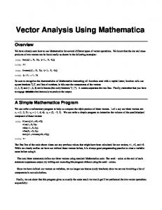
We can show that the optimal hyperplane, defined as the one with the maximal margin of separation between the two classes (see Fig. 1), has the lowest capacity, which ensuring that the classifier learned from training samples will misclassify the less elements of the test samples originated from the same probability distribution.

x1 x2

γ

Fig. 1. A separable classification problem. The optimal hyperplane is orthogonal to the shortest line connecting the convex hulls of the two classes, and intersects it half way. There is a weight vector w and a threshold b such that yi ( w, xi + b ) > 0 . Rescaling w and b such

that the point(s) closest to the hyperplane satisfy

w, xi + b = 1 , we obtain a form (w, b) of

the hyperplane with yi ( w, xi + b ) ≥ 1 . Note that the margin, measured perpendicularly to the hyperplane, equals 1 / w . To maximize the margin, we thus have to minimize w subject to yi ( w, xi + b ) ≥ 1 [2].

1.3 Maximal margin classifier The optimization problem to find the optimal w vector and the threshold b is the following, given a set of linearly separable training samples S = (( x1 , y1 ), ..., ( xm , ym )) the hyperplane ( w∗ , b ∗ ) that maximizes the geometric margin. minimizew,b w, w subject to yi w, xi + b ≥ 1, i = 1, ... m .

Then the geometric margin can be computed considering that

w∗ , x1 + b∗ = 1

w ∗ , x 2 + b ∗ = −1 then w∗ , ( x1 − x2 ) = 2 rescaling w∗ 2 , ( x1 − x2 ) = ∗ ∗ w w

therefore the margin is 1 . w∗

γ=

The training patterns lie closest to the hyperplane (see Fig. 1 two balls and one diamond) are called support vectors, carrying all relevant information about the classification problem. The number of support vectors, SV are equal or less than the number of the training patterns, m. This minimization problem can be transformed into a dual maximization problem leading to a quadratic programming task, whose solution w has an expansion SV

w = ∑ vi xi i =1

Consequently, the final decision function is

 SV  f ( x) = sign  ∑ vi x, xi + b   i =1  which depends only on dot products between patterns. This lets us generalize to the nonlinear case. 1.4 Feature spaces and kernels The Fig. 2 shows the basic idea of SV machines, which is to map the data into some other dot space, called the feature space F via nonlinear map,

Φ : Rn → F

and perform the above linear algorithm in F. This is only requires the evaluation of dot products, K (u , v) = Φ (u ),Φ (v)

Φ

X

F

Φ (x) o

x x o

o

Φ (o) Φ (x) Φ (o)

x

Φ (x)

Φ (o)

Fig. 2. The idea of SV machines: map the training data nonlinearly into a higher dimensional feature space via Φ, and construct a separating hyperplane with maximum margin there. This yields a nonlinear decision boundary in input space. By the use of kernel function, it is possible to compute the separating hyperplane without explicitly carrying out the map into the feature space [3].

Clearly, if F is high dimensional, the dot product on the right hand side will be very expensive to compute. In some cases, however there is a simple kernel that can be evaluated efficiently. For instance, the polynomial kernel K (u, v) = u, v

d

can be shown to correspond to a map Φ into the space spanned by all products of exactly d dimensions of R n . For d = 2 and u, v ∈ R 2 , for example, we have

u, v

2

 =  

 u1   v1   ,    u 2   v2 

 u12   v12  2       =  2 u1u 2 ,  2 v1v2  = Φ (u ), Φ (v)   u2   v2   2 2    

defining Φ ( x) = ( x12 , 2 x1 x2 , x22 ) . More generally, we can prove that for every kernel that gives rise to a positive matrix (kernel matrix) M ij = K ( xi , x j ) , we can construct a map such that K (u , v) = Φ (u ),Φ (v) holds.

1.5 Optimization as a dual quadratic programming problem Now the dual minimization problem of margin maximization is the following, consider classifying a set of training samples, S = (( x1 , y1 ), ... ( xm , ym ))

using the feature space implicitly defined by the kernel K ( x, z ) and suppose the parameters α ∗ solve the following quadratic optimization problem, m

minimize W (α ) = ∑ α i − i =1

subject to

m

∑ yα i =1

i

i

1 m 1   yi y jα iα j  K ( xi , x j ) + δ ij  ∑ 2 i , j =1 c  

= 0, α i ≥ 0, i = 1, ... m .

m

α i∗

i =1

c

Let f ( x) = ∑ yiα i∗ K ( xi , x) + b∗ , where b∗ is chosen so that yi f ( xi ) = 1 −

for any

i with α i∗ ≠ 0 . Then the decision rule given by sign ( f ( x)) is equivalent to the hyperplane in the feature space implicitly defined by the kernel K ( x, z ) , which solves the optimization problem, where the geometric margin is   1 γ =  ∑ α i∗ − α ∗ , α ∗  c  i∈sv 

−1

2

where set sv corresponds to indexes i, for which α i∗ ≠ 0 ,

{

}

sv = i : α i∗ ≠ 0; i = 1, ... m

Training samples, xi for which i ∈ sv are called support vectors giving contribution to the definition of f ( x) .

2 Implementation of SVC in Mathematica

2.1 Steps of implementation

The dual optimization problem can be solved conveniently using Mathematica. In this section, the steps of the implementation of SVC algorithm are shown by solving XOR problem. The truth table of XOR, using bipolar values for the output, is Table 1. Truth table of XOR problem

x1 0 0 1 1

x2 0 1 0 1

The input and output data lists are xym={{0,0},{0,1},{1,0},{1,1}}; zm={-1,1,1,-1};

Let us employ Gaussian kernel with β gain β=10.;

y -1 1 1 -1

K[u_,v_]:=Exp[-β (u-v).(u-v)]

The number of the data pairs in the training set, m is m=Length[zm] 4

Create the objective function W (α ) to be maximized, with regularization parameter, c=5.;

First, we prepare a matrix M, which is an extended form of the kernel matrix, M=(Table[N[K[xym[[i]],xym[[j]]]], {i,1,m},{j,1,m}]+(1/c)IdentityMatrix[m]);

then the objective function can be expressed as, m

W= ∑ αi –(1/2) i= 1

m

∑

m

∑ (zm[[i]]zm[[j]] αi αj M[[i,j]]);

i=1 j=1

The constrains for the unknown variables are g=Apply[And,Join[Table[αi ≥0,{i,1,m}],{

m

∑ zm[[i]]αim0}]];

i=1

However the maximization problem is a convex quadratic problem, from practical reasons to maximize the objective function the built in function NMaximize is applied. NMaximize implements several algorithms for finding constrained global optima. The methods are flexible enough to cope with functions that are not differentiable or continuous, and are not easily trapped by local optima. Possible settings for the Method option include "RandomSearch", "NelderMead", "DifferentialEvolution" and "SimulatedAnnealing". Here we use DifferentialEvolution, which is a genetic algorithm that maintains a population of specimens, x1 , ..., xn , represented as vectors of real numbers (“genes”). Every iteration, each xi chooses random integers a, b, and c and constructs the mate yi = xi + γ ( xa + ( xb − xc )) , where γ is the value of ScalingFactor. Then xi is mated with yi according to the value of CrossProbability, giving us the child zi . At this point xi competes against zi for the position of xi in the population. The default value of SearchPoints is Automatic, which is Min[10*d, 50], where d is the number of variables. We need the list of unknown variables α , vars=Table[αi,{i,1,m}];

Then the solution of the maximization problem is, sol=NMaximize[{W,g},vars,Method→DifferentialEvolution] {1.66679,{α1→0.833396, α2→0.833396, α3→0.833396, α4→0.833396}}

The consistency of this solution can be checked by computing values of b for every data points. Theoretically, these values should be same for any data points, however, in general, this is only approximately true. bdata=Table[((1-αj/c)/zm[[j]]m

∑ zm[[i]]αi K[xym[[i]],xym[[j]]])/.sol[[2]],{j,1,m}]

i= 1

{-1.89729×10-16, 6.65294×10-17, 3.45251×10-16, 0.}

The value of b can be chosen as the average of these values b=Apply[Plus,bdata]/m 5.55126×10-17

Then the classifier function is, f[w_]:=((

m

∑ zm[[i]]αiK[w,xym[[i]]])+b)/.sol[[2]]

i= 1

In symbolic form Clear[x,y] f[{x,y}] 2 2 2 2 5.55126×10-17-0.833396 e-10.((-1+x) +(-1+y) ) +0.833396 e-10.(x +(-1+y) ) 2 2 2 2 +0.833396 e-10.((-1+x) +y ) -0.833396 e-10.(x +y )

Let us display the contour lines of the continuous classification function,