SSVM: A Smooth Support Vector Machine for Classification Yuh-Jye Lee and O. L. Mangasarian Computer Sciences Department University of Wisconsin 1210 West Dayton Street Madison, WI 53706
[email protected],
[email protected]
Abstract Smoothing methods, extensively used for solving important mathematical programming problems and applications, are applied here to generate and solve an unconstrained smooth reformulation of the support vector machine for pattern classification using a completely arbitrary kernel. We term such reformulation a smooth support vector machine (SSVM). A fast Newton-Armijo algorithm for solving the SSVM converges globally and quadratically. Numerical results and comparisons are given to demonstrate the effectiveness and speed of the algorithm. On six publicly available datasets, tenfold cross validation correctness of SSVM was the highest compared with four other methods as well as the fastest. On larger problems, SSVM was comparable or faster than SVMlight [17], SOR [23] and SMO [27]. SSVM can also generate a highly nonlinear separating surface such as a checkerboard.
1
Introduction
Smoothing methods have been extensively used for solving important mathematical programming problems [8, 9, 7, 10, 11, 16, 29, 13]. In this paper, we introduce a new formulation of the support vector machine with linear (5) 1
and nonlinear kernel (24) [30, 5, 6, 21] for pattern classification. We begin with the linear case which can be converted to an unconstrained optimization problem (7). Since the objective function of this unconstrained optimization problem is not twice differentiable, we employ a smoothing technique to introduce the smooth support vector machine (SSVM) (9). The smooth support vector machine has important mathematical properties such as strong convexity and infinitely often differentiability. Based on these properties, we can prove that when the smoothing parameter α in the SSVM approaches infinity, the unique solution of the SSVM converges to the unique solution of the original optimization problem (5). We also prescribe a Newton-Armijo algorithm (i.e. a Newton method with a stepsize determined by the simple Armijo rule which eventually becomes redundant) to solve the SSVM and show that this algorithm globally and quadratically converges to the unique solution of the SSVM. To construct a nonlinear classifier, a nonlinear kernel [30, 21] is used to obtain the nonlinear support vector machine (24) and its corresponding smooth version (25) with a completely arbitrary kernel. The smooth formulation (25) with a nonlinear kernel retains the strong convexity and twice differentiability and thus we can apply Newton-Armijo algorithm to solve it. We briefly outline the contents of the paper now. In Section 2 we state the pattern classification problem and derive the smooth unconstrained support vector machine (9) from a constrained optimization formulation (5). Theorem 2.2 shows that the unique solution of our smooth approximation problem (9) will approach the unique solution of the original unconstrained optimization problem (7) as the smoothing parameter α approaches infinity. A Newton-Armijo Algorithm 3.1 for solving the SSVM converges globally and quadratically as shown in Theorem 3.2. In Section 4 we extend the SSVM to construct a nonlinear classifier by using a nonlinear kernel. All the Newton-Armijo convergence results apply to this nonlinear kernel formulation. Numerical tests and comparisons are given in Section 5. For moderate sized datasets, SSVM gave the highest tenfold cross validation correctness on six publicly available datasets as well as the fastest times when compared with four other methods given in [2, 4]. To demonstrate SSVM’s capability in solving larger problems we compared SSVM with successive overrelaxation (SOR) algorithm [23], sequential minimal optimization (SMO) algorithm [27] and SVMlight [17] on the Irvine Machine Learning Database Repository Adult dataset [26]. It turns out that SSVM with a linear kernel is very efficient for this large dataset. By using a nonlinear kernel, SSVM can obtain very sharp 2
separation for the highly nonlinear checkerboard pattern of [18] as depicted in Figures 4 and 5. To make this paper self-contained, we state and prove a Global Quadratic Convergence Theorem for the Newton-Armijo method in the Appendix which is employed in Theorem 3.2. A word about our notation and background material. All vectors will be column vectors unless transposed to a row vector by a prime superscript ′ . For a vector x in the n-dimensional real space Rn , the plus function x+ is defined as (x+ )i = max {0, xi }, i = 1, . . . , n. The scalar (inner) product of two vectors x and y in the n-dimensional real space Rn will be denoted by x′ y and the p-norm of x will be denoted by kxkp . For a matrix A ∈ Rm×n , Ai is the ith row of A which is a row vector in Rn . A column vector of ones of arbitrary dimension will be denoted by e. We shall employ the MATLAB “dot” notation [25] to signify application of a function to all components of a matrix or a vector. For example if A ∈ Rm×n , then A2• ∈ Rm×n will denote the matrix obtained by squaring each element of A. For A ∈ Rm×n and B ∈ Rn×l , the kernel K(A, B) maps Rm×n × Rn×l into Rm×l . In particular, if x and y are column vectors in Rn then, K(x′ , y) is a real number, K(x′ , A′ ) is a row vector in Rm and K(A, A′ ) is an m × m matrix. If f is a real valued function defined on the n-dimensional real space Rn , the gradient of f at x is denoted by ∇f (x) which is a row vector in Rn and the n × n Hessian matrix of second partial derivatives of f at x is denoted by ∇2 f (x). The level set of f is defined as Lµ (f ) = {x|f (x) ≤ µ} for a given real number µ. The base of the natural logarithm will be denoted by ε.
2
The Smooth Support Vector Machine (SSVM)
We consider the problem of classifying m points in the n-dimensional real space Rn , represented by the m × n matrix A, according to membership of each point Ai in the classes 1 or -1 as specified by a given m × m diagonal matrix D with ones or minus ones along its diagonal. For this problem the standard support vector machine with a linear kernel AA′ [30, 12] is given by the following for some ν > 0: min
(w,γ,y)∈Rn+1+m
νe′ y + 21 w ′w
s.t. D(Aw − eγ) + y ≥ e y ≥ 0.
3
(1)
Here w is the normal to the bounding planes: x′ w − γ = +1 x′ w − γ = −1,
(2)
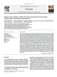
and γ determines their location relative to the origin. The first plane above bounds the class 1 points and the second plane bounds the class -1 points when the two classes are strictly linearly separable, that is when the slack variable y = 0. The linear separating surface is the plane x′ w = γ,
(3)
midway between the bounding planes (2). See Figure 1. If the classes are linearly inseparable then the two planes bound the two classes with a “soft margin” determined by a nonnegative slack variable y, that is: x′ w − γ + yi ≥ +1, for x′ = Ai and Dii = +1, x′ w − γ − yi ≤ −1, for x′ = Ai and Dii = −1.
(4)
The 1-norm of the slack variable y is minimized with weight ν in (1). The quadratic term in (1), which is twice the reciprocal of the square of the 2-norm 2 distance kwk between the two bounding planes of (2) in the n-dimensional 2 space of w ∈ Rn for a fixed γ, maximizes that distance, often called the “margin”. Figure 1 depicts the points represented by A, the bounding planes 2 (2) with margin kwk , and the separating plane (3) which separates A+, 2 the points represented by rows of A with Dii = +1, from A−, the points represented by rows of A with Dii = −1. In our smooth approach, the square of 2-norm of the slack variable y is minimized with weight ν2 instead of the 1-norm of y as in (1). In addition the distance between the planes (2) is measured in the (n + 1)-dimensional 2 space of (w, γ) ∈ Rn+1 , that is k(w,γ)k . Measuring the margin in this (n + 1)2 n dimensional space instead of R induces strong convexity and has little or no effect on the problem as was shown in [23]. Thus using twice the reciprocal squared of the margin instead, yields our modified SVM problem as follows: min
w,γ,y
s.t.
ν ′ yy 2
+ 12 (w ′ w + γ 2 )
D(Aw − eγ) + y ≥ e y ≥ 0.
(5)
At a solution of problem (5), y is given by y = (e − D(Aw − eγ))+ , 4
(6)
x′ w = γ + 1 x
x x x
x
x
x x x x x x x x
A+
x x x x A- x x x x x x x x x′ w = γ − 1
Margin=
2 kwk2
w
Separating Surface: x′ w = γ Figure 1: The bounding planes (2) with margin
2 kwk2 ,
and the plane (3) separating A+, the points represented by rows of A with Dii = +1, from A−, the points represented by rows of A with Dii = −1.
where, as defined earlier, (·)+ replaces negative components of a vector by zeros. Thus, we can replace y in (5) by (e − D(Aw − eγ))+ and convert the SVM problem (5) into an equivalent SVM which is an unconstrained optimization problem as follows: min w,γ
ν k(e 2
− D(Aw − eγ))+ k22 + 21 (w ′ w + γ 2 ).
(7)
This problem is a strongly convex minimization problem without any constraints. It is easy to show that it has a unique solution. However, the objective function in (7) is not twice differentiable which precludes the use of a fast Newton method. We thus apply the smoothing techniques of [8, 9] and replace x+ by a very accurate smooth approximation (see Lemma 2.1 below) that is given by p(x, α), the integral of the sigmoid function 1+ε1−αx of neural networks [19], that is p(x, α) = x +
1 log(1 + ε−αx ), α > 0. α
(8)
This p function with a smoothing parameter α is used here to replace the 5
plus function of (7) to obtain a smooth support vector machine (SSVM) : 1 ν minn+1 kp(e − D(Aw − eγ), α)k22 + (w ′w + γ 2 ). (w,γ)∈R (w,γ)∈R 2 2 (9) We will now show that the solution of problem (5) is obtained by solving problem (9) with α approaching infinity. We take advantage of the twice differentiable property of the objective function of (9) to utilize a quadratically convergent algorithm for solving the smooth support vector machine (9). We begin with a simple lemma that bounds the square difference between the plus function (x)+ and its smooth approximation p(x, α). minn+1 Φα (w, γ) :=
Lemma 2.1 For x ∈ R and |x| < ρ : p(x, α)2 − (x+ )2 ≤ ( logα 2 )2 + 2ρ log 2, α where p(x, α) is the p function of (8) with smoothing parameter α > 0. Proof We consider two cases. For 0 < x < ρ, 2x 1 log2 (1 + ε−αx ) + log(1 + ε−αx ) 2 α α log 2 2 2ρ ≤ ( ) + log 2. α α
p(x, α)2 − (x+ )2 =
For −ρ < x ≤ 0, p(x, α)2 is a monotonically increasing function, so we have p(x, α)2 − (x+ )2 = p(x, α)2 ≤ p(0, α)2 = ( Hence, p(x, α)2 − (x+ )2 ≤ ( logα 2 )2 +
2ρ α
log 2 2 ) . α
log 2. 2
We now show that as the smoothing parameter α approaches infinity the unique solution of our smooth problem (9) approaches the unique solution of the equivalent SVM problem (7). We shall do this for a function f (x) given in (10) below that subsumes the equivalent SVM function of (7) and for a function g(x, α) given in (11) below which subsumes the SSVM function of (9). Theorem 2.2 Let A ∈ Rm×n and b ∈ Rm×1 . Define the real valued functions f (x) and g(x, α) in the n-dimensional real space Rn : 1 1 f (x) = k(Ax − b)+ k22 + kxk22 2 2 6
(10)
and
1 1 g(x, α) = kp((Ax − b), α)k22 + kxk22 , 2 2
(11)
with α > 0. (i) There exists a unique solution x¯ of minn f (x) and a unique solution x¯α x∈R
of minn g(x, α). x∈R
(ii) For all α > 0, we have the following inequality: k¯ xα − x¯k22 ≤
m log 2 2 log 2 (( ) + 2ξ ), 2 α α
(12)
max |(A¯ x − b)i |.
(13)
where ξ is defined as follows: ξ =
1≤i≤m
Thus, x¯α converges to x¯ as α goes to infinity with an upper bound given by (12). Proof (i) To show the existence of unique solutions, we know that since x+ ≤ p(x, α), the level sets Lν (g(x, α)) and Lν (f (x)) satisfy Lν (g(x, α)) ⊆ Lν (f (x)) ⊆ {x|kxk22 ≤ 2ν},
(14)
for ν ≥ 0. Hence Lν (g(x, α)) and Lν (f (x)) are compact subsets in Rn and the problems minn f (x) and minn g(x, α) have solutions. By the strong convexity x∈R
x∈R
of f (x) and g(x, α) for all α > 0, these solutions are unique. (ii) To establish convergence, we note that by the first order optimality condition and strong convexity of f (x) and g(x, α) we have that 1 1 f (¯ xα ) − f (¯ x) ≥ ∇f (¯ x)(¯ xα − x¯) + k¯ xα − x¯k22 = k¯ xα − x¯k22 , 2 2
(15)
1 1 g(¯ x, α) − g(¯ xα , α) ≥ ∇g(¯ xα , α)(¯ x − x¯α ) + k¯ x − x¯α k22 = k¯ x − x¯α k22 . (16) 2 2 Since the p function dominates the plus function we have that g(x, α)−f (x) ≥ 0 for all α > 0. Adding (15) and (16) and using this fact gives: k¯ xα − x¯k22 ≤ (g(¯ x, α) − f (¯ x)) − (g(¯ xα , α) − f (¯ xα )) ≤ g(¯ x, α) − f (¯ x) 1 = 2 kp((A¯ x − b), α)k22 − 21 k(A¯ x − b)+ k22 . 7
(17)
Application of Lemma 2.1 gives: k¯ xα − x¯k22 ≤
m log 2 2 (( α ) 2
+ 2ξ logα 2 ),
(18)
where ξ is a fixed positive number defined in (13). The last term in (18) will converge to zero as α goes to infinity. Thus x¯α converges to x¯ as α goes to infinity with an upper bound given by (12). 2 We will now describe a Newton-Armijo algorithm for solving the smooth problem (9).
3
A Newton-Armijo Algorithm for the Smooth Support Vector Machine
By making use of the results of the previous section and taking advantage of the twice differentiability of the objective function of problem (9), we prescribe a quadratically convergent Newton algorithm with an Armijo stepsize [1, 15, 3] that makes the algorithm globally convergent. Algorithm 3.1 Newton-Armijo Algorithm for SSVM (9) Start with any (w 0 , γ 0 ) ∈ Rn+1 . Having (w i , γ i), stop if the gradient of the objective function of (9) is zero, that is ∇Φα (w i, γ i ) = 0. Else compute (w i+1, γ i+1 ) as follows: (i) Newton Direction: Determine direction di ∈ Rn+1 by setting equal to zero the linearization of ∇Φα (w, γ) around (w i , γ i) which gives n + 1 linear equations in n + 1 variables: ∇2 Φα (w i , γ i)di = −∇Φα (w i, γ i )′ .
(19)
(ii) Armijo Stepsize [1]: Choose a stepsize λi ∈ R such that: (w i+1 , γ i+1 ) = (w i , γ i ) + λi di
(20)
where λi = max{1, 21 , 41 , . . .} such that : Φα (w i , γ i ) − Φα ((w i , γ i ) + λi di ) ≥ −δλi ∇Φα (w i, γ i )di where δ ∈ (0, 12 ). 8
(21)
Note that a key difference between our smoothing approach and that of the classical SVM [30, 12] is that we are solving here a linear system of equations (19) instead of solving a quadratic program as is the case with the classical SVM. Furthermore, we can show that our smoothing Algorithm 3.1 converges globally to the unique solution and takes a pure Newton step after a finite number of iterations. This leads to the following quadratic convergence result: Theorem 3.2 Let {(w i, γ i )} be a sequence generated by Algorithm 3.1 and (w, ¯ γ¯ ) be the unique solution of problem (9). (i) The sequence {(w i, γ i )} converges to the unique solution (w, ¯ γ¯ ) from any initial point (w 0 , γ 0 ) in Rn+1 . (ii) For any initial point (w 0, γ 0 ), there exists an integer ¯i such that the stepsize λi of Algorithm 3.1 equals 1 for i ≥ ¯i and the sequence {(w i, γ i )} converges to (w, ¯ γ¯ ) quadratically. Although this theorem can be inferred from [15, Therem 6.3.4, pp 123125], we give its proof in the Appendix for the sake of completeness. We note here that even though the Armijo stepsize is needed to guarantee that Algorithm 3.1 is globally convergent, in most of our numerical tests Algorithm 3.1 converged from any starting point without the need for an Armijo stepsize.
4
SSVM with a Nonlinear Kernel
In Section 2 the smooth support vector machine formulation constructed a linear separating surface (3) for our classification problem. We now describe how to construct a nonlinear separating surface which is implicitly defined by a kernel function. We briefly describe now how the generalized support vector machine (GSVM) [21] generates a nonlinear separating surface by using a completely arbitrary kernel. The GSVM solves the following mathematical program for a general kernel K(A, A′ ): min u,γ,y
νe′ y + f (u)
s.t. D(K(A, A′ )Du − eγ) + y ≥ e y ≥ 0. 9
(22)
Here f (u) is some convex function on Rm which suppresses the parameter u and ν is some positive number that weights the classification error e′ y versus the suppression of u. A solution of this mathematical program for u and γ leads to the nonlinear separating surface K(x′ , A′ )Du = γ
(23)
The linear formulation (1) of Section 2 is obtained if we let K(A, A′ ) = AA′ , w = A′ Du and f (u) = 21 u′ DAA′ Du. We now use a different classification objective which not only suppresses the parameter u but also suppresses γ in our nonlinear formulation: min u,γ,y
ν ′ yy 2 ′
+ 21 (u′ u + γ 2 )
s.t. D(K(A, A )Du − eγ) + y ≥ e y ≥ 0.
(24)
We repeat the same arguments as in Section 2 to obtain the SSVM with a nonlinear kernel K(A, A′ ): min u,γ
ν kp(e 2
− D(K(A, A′ )Du − eγ), α)k22 + 21 (u′u + γ 2 ),
(25)
where K(A, A′ ) is a kernel map from Rm×n × Rn×m to Rm×m . We note that this problem, which is capable of generating highly nonlinear separating surfaces, still retains the strong convexity and differentiability properties for any arbitrary kernel. All of the results of the previous sections still hold. Hence we can apply the Newton-Armijo Algorithm 3.1 directly to solve (25). We turn our attention now to numerical testing.
5
Numerical Results and Comparisons
We demonstrate now the effectiveness and speed of the smooth support vector machine (SSVM) approach by comparing it numerically with other methods. All parameters in the SSVM algorithm were chosen for optimal performance on a tuning set, a surrogate for a testing set. For a linear kernel, we divided the comparisons into two parts, moderate sized problems and larger problems. We also tested the ability of SSVM in generating a highly nonlinear separating surface. Although we established global and quadratic convergence of our Newton algorithm under an Armijo step-size rule, in practice 10
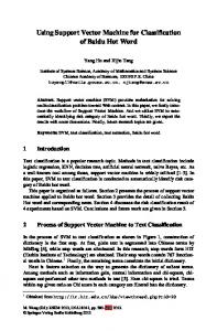
the Armijo stepsize was turned off in all numerical tests without any noticeable change. Furthermore, we used the limit values of the sigmoid function 1 and the p function (8) as the smoothing parameter α goes to infinity, 1+ε−αx that is the unit step function with value 21 at zero and the plus function (·)+ respectively, when we computed the Hessian matrix and the gradient in (19). This gave slightly faster computational times but made no difference in the computational results from those obtained with α = 5. All our experiments were run on the University of Wisconsin Computer Sciences Department Ironsides cluster. This cluster of four Sun Enterprise E6000 machines, each machine consists of 16 UltraSPARC II 250 MHz processors and 2 gigabytes of RAM, resulting in a total of 64 processors and 8 gigabytes of RAM. All linear and quadratic programming formulations were solved using the CPLEX package [14] called from within MATLAB [25]. In order to evaluate how well each algorithm generalizes to future data, we performed tenfold cross-validation on each dataset [28]. To evaluate the efficacy of SSVM, we compared computational times of SSVM with robust linear program (RLP) algorithm [2], the feature selection concave minimization (FSV) algorithm, the support vector machine using the 1-norm approach (SVMk·k1 ) and the classical support vector machine (SVMk·k22 ) [4, 30, 12]. We ran all tests on six publicly available datasets: the Wisconsin Prognostic Breast Cancer Database [24] and four datasets from the Irvine Machine Learning Database Repository [26]. It turned out that tenfold testing correctness of the SSVM is the highest for these five methods on all datasets tested as well as the computational speed. We summarize all these results in Table 1. We also tested SSVM on the Irvine Machine Learning Database Repository [26] Adult dataset to demonstrate the capability of SSVM in solving larger problems. Training set sizes varied from 1,605 to 32,562 training examples and each example included 123 binary attributes. We compared the results with RLP directly and SOR [23], SMO [27] and SVMlight [17] indirectly. The results show that SSVM not only has a very good testing set accuracy but also has low computational times. The results for SOR, SMO and SVMlight are quoted from [23]. We summarize these details in Table 2 and Figure 2. We also solved the Adult dataset with 1,605 training examples via a classical support vector machine approach. It took 1,695.4 seconds to solve the problem using the CPLEX quadratic programming solver which employs a barrier function method [14]. In contrast, SSVM took 1.9 seconds
11
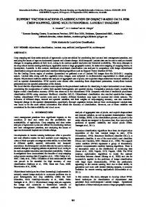
only to solve the same problem as indicated in Table 2. Figure 2 indicates that computational time grows almost linearly for SSVM whereas it grows at a faster rate for SOR and SMO. To test the effectiveness of the SSVM in generating a highly nonlinear separating surface, we tested it on the checkerboard dataset of [18] depicted in Figure 3. We used the following symmetric sixth degree polynomial kernel introduced in [23] as well a Gaussian kernel in the SSVM formulation (25): Polynomial Kernel : (( Aλ − ρ)( Aλ − ρ)′ − µ)d• Gaussian Kernel :
2
ε−µkAi −Aj k2 , i, j = 1, 2, 3 . . . m.
Values of the parameters λ, ρ, µ used are given in Figures 4 and 5 as well as that of the parameter ν of the nonlinear SSVM (25). The results are shown in Figures 4 and 5 . We note that the boundaries of the checkerboard are as sharp as those of [23], obtained by a linear programming solution, and considerably sharper than those of [18], obtained by a Newton approach applied to a quadratic programming formulation.
6
Conclusion and Future Work
We have proposed a new formulation, SSVM, which is a smooth unconstrained optimization reformulation of the traditional quadratic program associated with a SVM. SSVM is solved by a very fast Newton-Armijo algorithm and has been extended to nonlinear separation surfaces by using nonlinear kernel techniques. The numerical results show that SSVM is faster than other methods and has better generalization ability. Future work includes other smooth formulations, feature selection via SSVM and smooth support vector regression. We also plan to use the row and column generation chunking algorithms of [5, 22] in conjunction with SSVM to solve extremely large classification problems which do not fit in memory, for both linear and nonlinear kernels.
Acknowledgements The research described in this Data Mining Institute Report 99-03, September 1999, was supported by National Science Foundation Grants CCR-9729842 12
and CDA-9623632, by Air Force Office of Scientific Research Grant F4962097-1-0326 and by the Microsoft Corporation. Ten-Fold Training Correctness, % Ten-Fold Testing Correctness, % Ten-Fold Computational Time, sec. Dataset size Method m×n SSVM RLP SVMk·k1 SVMk·k22 WPBC(24 months) 155 × 32 WPBC(60 months) 110 × 32 Ionosphere 351 × 34 Cleveland 297 × 13 Pima Indians 768 × 8 BUPA Liver 345 × 6
86.16 83.47 2.32 80.20 68.18 1.03 94.12 89.63 3.69 87.32 86.13 1.63 78.11 78.12 1.54 70.37 70.33 1.05
85.23 67.12 6.47 87.58 63.50 2.81 94.78 86.04 10.38 86.31 83.87 12.74 76.48 76.16 195.21 68.98 64.34 17.26
74.40 71.08 6.25 71.21 66.23 3.72 88.92 86.10 42.41 85.30 84.55 18.71 75.52 74.47 286.59 67.83 64.03 19.94
81.94 82.02 12.50 80.91 61.83 4.91 92.96 89.17 128.15 72.05 72.12 67.55 77.92 77.07 1138.0 70.57 69.86 123.24
FSV 88.89 81.93 22.54 86.36 64.55 7.31 94.87 86.76 10.49 87.95 85.31 21.15 77.91 76.96 227.41 71.21 69.81 25.10
Table 1: Ten-fold cross-validation correctness results on six moderate sized datasets using five different methods. All linear and quadratic programming formulations were solved using the CPLEX package [14] called from within MATLAB [25]. Bold type indicates the best result.
13
Dataset size
Testing Correctness % Running Time Sec
(Training, Testing)
Method
n = no. of feature
SSVM
SOR
SMO
(1605, 30957) n = 123 (2265, 30297) n = 123 (3185, 29377) n = 123 (4781, 27781) n = 123 (6414, 26148) n = 123 (11221, 21341) n = 123 (16101, 16461) n = 123 (22697, 9865) n = 123 (32562, 16282) n = 123
84.27 1.9 84.57 2.8 84.63 3.9 84.55 6.0 84.60 8.1 84.79 14.1 84.96 21.5 85.35 29.0 85.02 44.5
84.06 0.3 0.4 84.24 1.2 0.9 84.23 1.4 1.8 84.28 1.6 3.6 84.30 4.1 5.5 84.37 18.8 17.0 84.62 24.8 35.3 85.06 31.3 85.7 84.96 83.9 163.6
SVMlight
RLP
84.25 5.4 84.43 10.8 84.40 21.0 84.47 43.2 84.43 87.6 84.68 306.6 84.83 667.2 85.17 1425.6 85.05 2184.0
78.68 9.9 77.19 19.12 77.83 80.1 79.15 88.6 71.85 218.8 60.00 449.2 72.52 632.6 77.43 991.9 83.25 1561.1
Table 2: Testing set correctness results on the larger Adult dataset obtained by five different methods. The SOR, SMO and SVMlight are from [23]. The SMO experiments were run on a 266 MHz Pentium II processor under Windows NT 4 and using Microsoft’s Visual C++ 5.0 compiler. The SOR experiments were run on a 200 MHz Pentium Pro with 64 megabytes of RAM, also under Windows NT 4 and using VisualC++ 5.0. The SVMlight experiments were run on the same hardware as that for SOR, but under the Solaris 5.6 operating system. Bold type indicates the best result and a dash (-) indicates that the results were not available from [23].
14
180 SSVM SOR SMO
160
140
Time (CPU sec.)
120
100
80
60
40
20
0
0
5000
10000
15000 20000 Training set size
25000
30000
35000
Figure 2: Comparison of SSVM, SOR and SMO on the larger Adult dataset. Note the essentially linear time growth of SSVM. 200
180
160
140
120
100
80
60
40
20
0
0
20
40
60
80
100
120
140
160
180
Figure 3: The checkerboard training dataset 15
200
200
180
160
140
120
100
80
60
40
20
0
0
20
40
60
80
100
120
140
160
180
200
Figure 4: Indefinite sixth degree polynomial kernel separation of the checkerboard dataset (ν = 320, 000, λ = 100, ρ = 1, d = 6, µ = 0.5) 200
180
160
140
120
100
80
60
40
20
0
0
20
40
60
80
100
120
140
160
180
200
Figure 5: Gaussian kernel separation of he checkerboard dataset (ν = 10, µ = 2) 16
Appendix We establish here global quadratic convergence for a Newton-Armijo Algorithm for solving the unconstrained minimization problem: min f (x),
x∈Rn
(26)
where f is a twice differentiable real valued function on Rn satisfying conditions (i) and (ii) below. This result, which can also be deduced from [15, Theorem 6.3.4, pp 123-125] is given here for completeness. Newton-Armijo Algorithm for Unconstrained Minimization Let f be a twice differentiable real valued function on Rn . Start with any x0 ∈ Rn . Having xi , stop if the gradient of f at xi is zero, that is ∇f (xi ) = 0. Else compute xi+1 as follows: (i) Newton Direction: Determine direction di ∈ Rn by setting equal to zero, the linearization of ∇f (x) around xi which gives n linear equations in n variables: ∇2 f (xi )di = −∇f (xi )′ . (27) (ii) Armijo Stepsize [1]: Choose a stepsize λi ∈ R such that: xi+1 = xi + λi di
(28)
where λi = max{1, 12 , 41 , . . .} such that : f (xi ) − f (xi + λi di ) ≥ −δλi ∇f (xi )di
(29)
where δ ∈ (0, 21 ). Global Quadratic Convergence Theorem Let f be a twice differentiable real valued function on Rn and such that : (i) k∇2 f (y) − ∇2 f (x)k2 ≤ κky − xk2 , for all x, y ∈ Rn and some κ > 0, (ii) y∇2f (x)y ≥ µkyk22, for all x, y ∈ Rn and some µ > 0. Let {xi } be a sequence generated by the Newton-Armijo Algorithm. Then: (a) The sequence {xi } converges to x¯ such that ∇f (¯ x) = 0, where x¯ is the n unique global minimizer of f on R . 17
(b) kxi+1 − x¯k2 ≤
κ kxi 2µ
− x¯k22 , for i ≥ ¯i for some ¯i.
Proof (a) Since f (xi ) − f (xi+1 ) ≥ δλi ∇f (xi )∇2 f (xi )−1 ∇f (xi )′ ≥ 0,
(30)
the sequence {xi } is contained in the compact level set: Lf (x0 ) (f (x)) ⊆ {x| kx − x0 k2 ≤
2 k∇f (x0 )k2 }. µ
(31)
Hence y∇2f (xi )y ≤ νkyk22 , for all i = 0, 1, 2, . . . , y ∈ Rn , for some ν > 0.
(32)
It follows that −∇f (xi )di = ∇f (xi )∇2 f (xi )−1 ∇f (xi )′ ≥
1 k∇f (xi )k2 , ν
(33)
and by Theorem 2.1, Example 2.2 (iv) of [20] we have that each accumulation point of {xi } is stationary. Since all accumulation points of {xi } are identical to the global unique minimizer of the strongly convex function f , it follows that {xi } converges to x¯ such that ∇f (¯ x) = 0 and x¯ is the unique global minimizer of f on Rn . (b) We first show that the Armijo inequality holds from a certain i0 onward with λi = 1. Suppose not, then there exists a subsequence {xij } such that f (xij ) − f (xij + dij ) < −δ∇f (xij )dij , dij = −∇2 f (xij )−1 ∇f (xij )′ .
(34)
By the twice differentiability of f : 1 ′ f (xij + dij ) − f (xij ) = ∇f (xij )dij + dij ∇2 f (xij + tij dij )dij , 2
(35)
for some tij ∈ (0, 1). Hence 1 ′ −∇f (xij )dij − dij ∇2 f (xij + tij dij )dij < −δ∇f (xij )dij . 2
(36)
Collecting terms and substitution for dij gives: − 12 ∇f (xij )∇2 f (xij )−1 ∇2 f (xij + tij dij )∇2 f (xij )−1 ∇f (xij )′ < −(1 − δ)∇f (xij )∇2 f (xij )−1 ∇f (xij )′ . 18
(37)
Dividing by k∇f (xij )k22 and letting j go to infinity gives: 1 x)−1 q¯′ ≤ −(1 − δ)¯ q ∇2 f (¯ x)−1 q¯′ , − q¯∇2 f (¯ 2 or
1 ( − δ)¯ q ∇2 f (¯ x)−1 q¯′ ≤ 0, 2
(38)
∇f (xij ) where q¯ = lim . j→∞ k∇f (xij )k2 This contradicts the positive definiteness of ∇2 f (¯ x) for δ ∈ (0, 12 ). Hence for i ≥ ¯i for some ¯i, we have a pure Newton iteration, that is xi+1 = xi − ∇2 f (xi )−1 ∇f (xi )′ , i ≥ ¯i.
(39)
By part (a) above {xi } converges to x¯, such that ∇f (¯ x) = 0. We now establish the quadratic rate given by the inequality in (b). Since for i ≥ ¯i: t=1
xi+1 − x¯ = xi − x¯ − ∇2 f (xi )−1 [∇f (¯ x + t(xi − x¯))]t=0 R1 = (xi − x¯) − ∇2 f (xi )−1 0 (∇2 f (¯ x + t(xi − x¯) − ∇2 f (xi ) + ∇2 f (xi ))(xi − x¯)dt, (40) we have, upon cancelling the terms (xi − x¯) inside and outside the integral sign and taking norms, that : kxi+1 − x¯k2 ≤ k∇2 f (xi )−1 k2
R1
k∇2 f (¯ x + t(xi − x¯) − ∇2 f (xi )k2 kxi − x¯k2 dt R1 ≤ k∇2 f (xi )−1 k2 kxi − x¯k2 0 κ(1 − t)kxi − x¯k2 dt =
κ kxi 2µ
0
− x¯k22 .
2 (41)
References [1] L. Armijo. Minimization of functions having Lipschitz-continuous first partial derivatives. Pacific Journal of Mathematics, 16:1–3, 1966. [2] K. P. Bennett and O. L. Mangasarian. Robust linear programming discrimination of two linearly inseparable sets. Optimization Methods and Software, 1:23–34, 1992. 19
[3] D. P. Bertsekas. Nonlinear Programming. Athena Scientific, Belmont, MA, second edition, 1999. [4] P. S. Bradley and O. L. Mangasarian. Feature selection via concave minimization and support vector machines. In J. Shavlik, editor, Machine Learning Proceedings of the Fifteenth International Conference(ICML ’98), pages 82–90, San Francisco, California, 1998. Morgan Kaufmann. ftp://ftp.cs.wisc.edu/math-prog/tech-reports/98-03.ps. [5] P. S. Bradley and O. L. Mangasarian. Massive data discrimination via linear support vector machines. Optimization Methods and Software, 13:1–10, 2000. ftp://ftp.cs.wisc.edu/math-prog/tech-reports/98-03.ps. [6] C. J. C. Burges. A tutorial on support vector machines for pattern recognition. Data Mining and Knowledge Discovery, 2(2):121–167, 1998. [7] B. Chen and P. T. Harker. Smooth approximations to nonlinear complementarity problems. SIAM Journal of Optimization, 7:403–420, 1997. [8] Chunhui Chen and O. L. Mangasarian. Smoothing methods for convex inequalities and linear complementarity problems. Mathematical Programming, 71(1):51–69, 1995. [9] Chunhui Chen and O. L. Mangasarian. A class of smoothing functions for nonlinear and mixed complementarity problems. Computational Optimization and Applications, 5(2):97–138, 1996. [10] X. Chen, L. Qi, and D. Sun. Global and superlinear convergence of the smoothing Newton method and its application to general box constrained variational inequalities. Mathematics of Computation, 67:519– 540, 1998. [11] X. Chen and Y. Ye. On homotopy-smoothing methods for variational inequalities. SIAM Journal on Control and Optimization, 37:589–616, 1999. [12] V. Cherkassky and F. Mulier. Learning from Data - Concepts, Theory and Methods. John Wiley & Sons, New York, 1998. [13] P. W. Christensen and J.-S. Pang. Frictional contact algorithms based on semismooth newton methods. In Reformulation: Nonsmooth, Piecewise 20
Smooth, Semismooth and Smoothing Methods, M. Fukushima and L. Qi, (editors), pages 81–116, Dordrecht, Netherlands, 1999. Kluwer Academic Publishers. [14] CPLEX Optimization Inc., Incline Village, Nevada. Using the CPLEX(TM) Linear Optimizer and CPLEX(TM) Mixed Integer Optimizer (Version 2.0), 1992. [15] J. E. Dennis and R. B. Schnabel. Numerical Methods for Unconstrained Optimization and Nonlinear Equations. Prentice-Hall, Englewood Cliffs, N.J., 1983. [16] M. Fukushima and L. Qi. Reformulation: Nonsmooth, Piecewise Smooth, Semismooth and Smoothing Methods. Kluwer Academic Publishers, Dordrecht, The Netherlands, 1999. [17] T. Joachims. Making large-scale support vector machine learning practical. In Bernhard Sch¨olkopf, Christopher J. C. Burges, and Alexander J. Smola, editors, Advances in Kernel Methods - Support Vector Learning, pages 169–184. MIT Press, 1999. [18] L. Kaufman. Solving the quadratic programming problem arising in support vector classification. In Bernhard Sch¨olkopf, Christopher J. C. Burges, and Alexander J. Smola, editors, Advances in Kernel Methods - Support Vector Learning, pages 147–167. MIT Press, 1999. [19] O. L. Mangasarian. Mathematical programming in neural networks. ORSA Journal on Computing, 5(4):349–360, 1993. [20] O. L. Mangasarian. Parallel gradient distribution in unconstrained optimization. SIAM Journal on Control and Optimization, 33(6):1916–1925, 1995. ftp://ftp.cs.wisc.edu/tech-reports/reports/93/tr1145.ps. [21] O. L. Mangasarian. Generalized support vector machines. In A. Smola, P. Bartlett, B. Sch¨olkopf, and D. Schuurmans, editors, Advances in Large Margin Classifiers, pages 135–146, Cambridge, MA, 2000. MIT Press. ftp://ftp.cs.wisc.edu/math-prog/tech-reports/98-14.ps. [22] O. L. Mangasarian and David R. Musicant. Massive support vector regression. Technical Report 99-02, Data Mining Institute, Computer Sciences Department, University of Wisconsin, Madison, Wisconsin, July 21
1999. To appear in: “Applications and Algorithms of Complementarity”, M. C. Ferris, O. L. Mangasarian and J.-S. Pang, editors, Kluwer Academic Publishers,Boston 2000. ftp://ftp.cs.wisc.edu/pub/dmi/techreports/99-02.ps. [23] O. L. Mangasarian and David R. Musicant. Successive overrelaxation for support vector machines. IEEE Transactions on Neural Networks, 10:1032–1037, 1999. ftp://ftp.cs.wisc.edu/math-prog/tech-reports/9818.ps. [24] O. L. Mangasarian, W. N. Street, and W. H. Wolberg. Breast cancer diagnosis and prognosis via linear programming. Operations Research, 43(4):570–577, July-August 1995. [25] MATLAB. User’s Guide. The MathWorks, Inc., Natick, MA 01760, 1992. [26] P. M. Murphy and D. W. Aha. UCI repository of machine learning databases, 1992. www.ics.uci.edu/∼mlearn/MLRepository.html. [27] J. Platt. Sequential minimal optimization: A fast algorithm for training support vector machines. In Bernhard Sch¨olkopf, Christopher J. C. Burges, and Alexander J. Smola, editors, Advances in Kernel Methods - Support Vector Learning, pages 185–208. MIT Press, 1999. http://www.research.microsoft.com/∼jplatt/smo.html. [28] M. Stone. Cross-validatory choice and assessment of statistical predictions. Journal of the Royal Statistical Society, 36:111–147, 1974. [29] P. Tseng. Analysis of a non-interior continuation method based on chenmangasarian smoothing functions for complementarity problems. In Reformulation: Nonsmooth, Piecewise Smooth, Semismooth and Smoothing Methods, M. Fukushima and L. Qi, (editors), pages 381–404, Dordrecht, Netherlands, 1999. Kluwer Academic Publishers. [30] V. N. Vapnik. The Nature of Statistical Learning Theory. Springer, New York, 1995.
22


![A Support Vector Machine Classification Model for Benzo[c] - MDPI](https://m.moam.info/img/260x300/a-support-vector-machine-classification-model-for-_59f7b3ff1723dd71c04fbf69.jpg)