www.iosrjournals.org. 50 | Page. Support Vector Machine for Keratoconus Detection by Using. Topographic Maps with the Help of Image Processing Techniques.
IOSR Journal of Pharmacy and Biological Sciences (IOSR-JPBS) e-ISSN:2278-3008, p-ISSN:2319-7676. Volume 12, Issue 6 Ver. VI (Nov. – Dec. 2017), PP 50-58 www.iosrjournals.org
Support Vector Machine for Keratoconus Detection by Using Topographic Maps with the Help of Image Processing Techniques Alyaa H.Ali1., Nebras H.Ghaeb,2 Zahraa M.Musa1 1
Department of Physics/ College of science for women/ University of Baghdad/Iraq
Abstract: In recent years many researchers tried to find an accurate method to diagnose eye disease, researchers used different methods and devices for that. In this paper a method is present which depends on the details extracted from the topographic maps to detect Keratoconus (KC) that affects the cornea in diseased eye; with the help of image processing techniques. Twelve features (12) have been extracted from topographic maps collected from the Pentacam which is a device that acquired maps of the cornea and provide an information of the health of the eye, and applying these features to the support vector machine SVM (which is a supervised classification) to detect whether the cornea is healthy or diseased. Results showed that there is accuracy of about 90% for the tested data. Each normal indication will be written as Ok; and a Red flag will be written for the abnormal indications. Key Words: Image processing, Keratoconus (KC), SVM, Topographic Maps. ----------------------------------------------------------------------------------------------------------------------------- ---------Date of Submission: 11-12-2017 Date of acceptance: 30-12-2017 ----------------------------------------------------------------------------------------------------------------------------- ----------
I.
Introduction
The eye cornea is the outermost layer of the eye, it is the dome shaped clear surface that covers the front of the eye and plays an important role of focusing the vision. Although the cornea may seem clear and lacking of substance, but on the contrary, it is a highly organized tissue, unlike most tissues in the body, it contains no blood vessels to nourish and protect it from infections. Instead the cornea receive it nourishment from tears and from the aqueous humans (a fluid in the front part of the eye that lies behind the cornea) [1].The cornea can be affected by many diseases such as Fuchs' endothelial dystrophy, Bulbous keratopathy Glaucoma etc[2]. One of these diseases is Keratoconus; which is a non-inflammatory corneal disease that can be identified by locating a protrusion along with conical thinning in the cornea[3], as a result it will cause a distortion in vision. It is important to diagnose the effected cornea to give the right treatment for it; therefore researchers put their efforts to improve the software as well as hardware to present devices that gives accurate readings. There are different ways to detect KC[4]; the most used one is by using the Pentacam; which is a device that provide maps of the cornea as well as readings that gives information about the health of the cornea[5]. The Four Refractive maps are the maps that help to detect Keratoconus (KC), these maps contains from four maps (Sagittal, Pachymetric, Elevation front and Elevation back maps), each map gives an indication about the eye; and after revising all of the features from the four maps; decision will be made. There are some difficulties of diagnosing KC corneas; for the clinicians have to observe the maps that acquired from the device along with the reading and also, the results of examinations from other instruments to give the final decision; therefore, it is a very long complicating process. In the past years; researchers combine features that extracted from the maps with machine learning, such as Tout unchain et al.[6]employed 82 corneal maps and classified them into two groups normal and Keratoconus corneas ; 12 features of each map were extracted and used as an input for the classifiers, the classifiers that were used are NN, RBFNN, SVM and Decision Tree. Cheboli and Ravindran[7] proposed to use semi-supervised learner to label the un label data (clinically undiagnosed corneas). Souza et al. [8]. Proposed a way to estimate the performance of multi-layer perception, SVM and radial basis function neural network as contributory tools to recognise Keratoconus from maps that were taken from Orbscan II. This paper presented a method of diagnosing by using image processing and geometrical techniques to extract features from the four refractive maps provided by the Pentacam, and then entering these features to the SVM classifier to give an accurate diagnosing that support clinician opinion. In this work each normal indication will be written as ok; and a red flag will be written for the abnormal indications.
II. Methodology Data Collection: Data are acquired from Al-Amal Eye Private Clinic in Baghdad by using the Pentacam, where the cases are already examined and checked by the specialist doctors. The four refractive maps are used for this work; for they are the maps that are used to diagnose Keratoconus.
DOI: 10.9790/3008-1206065058
www.iosrjournals.org
50 | Page
Support Vector Machine for Keratoconus Detection by Using Topographic Maps with the Help of .. Subjects: 40 cases are used from both gender (22 females and 18 males), divided into two groups normal and abnormal. For each case the right corneal map (OD) is used. The range ages of the patents are between 54 to 20 years. Ten cases are used in this search.
III.
Application of Image Processing Techniques on The Maps:
This search focused on the four refractive maps because these are the maps that are used to detect KC. These maps are Sagittal map, Pachymetric map, Elevation map front and Elevation map back, each map can be acquired individually and also, all of them together as in figures(1, 2, 3, 4, and 5)
Fig. (1)The Four Refractive Maps.
Fig.(2) Individual Sagittal Map. DOI: 10.9790/3008-1206065058
www.iosrjournals.org
51 | Page
Support Vector Machine for Keratoconus Detection by Using Topographic Maps with the Help of ..
Fig.(3) Individual Pchymetric Map.
Fig. (4) Individual Elevation Map Front.
Fig.(5) Individual Elevation Map Back. DOI: 10.9790/3008-1206065058
www.iosrjournals.org
52 | Page
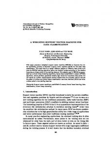
Support Vector Machine for Keratoconus Detection by Using Topographic Maps with the Help of .. The work is divided into five steps depending on each map and the applying techniques that are done on them. The features that are extracted from the four refractive maps are restricted in a circle with a diameter of 6mm; as it is the focal zone of the cornea and all changes will be happening inside this 6mm circle. Also, all maps are converted from RGB into gray level before extracting the features from them. SagittalMap: The features for the first three columns in table (1) represents the area of the bowtie shape, the area for the top half and the area for the bottom half respectively in the Sagittal map. A threshold has been applied to separate the shape from the background and calculating the area and knowing the value of the pixel for that area, then by dividing the bowtie shape from the centre of the map to count the area of each part as in figure (6) by using equation(1) [9].The area is counted in pixels. If there are big difference between the areas for both top and bottom halves then a red flag will be written as an indication of an abnormality.
(a) (b) Fig. (6) The threshold and separating the bowtie parts in Sagittal map where (a) is the top part (b) is the bottom part. 1 ≥ threshold then p = p + 1 G x, y = (1) 0 < threshold then P = 0 Where: G x, y : Is the threshold image [10]. Threshold : The threshold value of the pixel in the desired area. P : Is the area for the white pixel. The angle of skewing is a significant feature that need to be checked when examine the cornea. The angle of skewing for the Sagittal map has been counted in degree by fitting the horizontal and vertical meridians in the 6mm circle. A compass is fitted on the map after converting it into jpg (which is the same format as the maps to do merging between the compass and the maps). The slope which represents the skewing of the bowtie shape are applied by clicking on the two end of the skewed axes, then after knowing the slope; the angle is calculated using equations (2 and 3) [11], which shows the calculation of the slope and the angle of skewing. Then the angle of skewing is compared with the subjective axis (which is acquired from the clinic for the same patients from other instruments) as in figure (7). If the differences between the angle of skewing and the subjective axis for the same patients is more than 10 degree(according to the ophthalmologist) then there is a red flag which means that there is a risk of having KC, if not then it means it is ok.
Fig. (7) The angle of the skew in Sagittal Map after fitting the 6mm circle. Slope =(x2-x1)/ (y2-y1) (2) The angle = tan−1 slope (3) DOI: 10.9790/3008-1206065058
www.iosrjournals.org
53 | Page
Support Vector Machine for Keratoconus Detection by Using Topographic Maps with the Help of .. PachymetricMap: There are two features that are extracted from the Pachymetric map. First is the shape. As the Ophthalmologist familiar with; if the shape is circle like then there is red flag; and if the shape is more ellipse like then it is ok, after applying contour on the Pachymetric map to separate the concentric shapes from each other and then to be able to calculate the vertical and horizontal radius of the shape inside the 6mm circle as in equation (4,5) [10]. If both horizontal and vertical diameters for the shape are equal then it is a circle like and there is more indication of having Keratoconus, if not then the cornea is ok, as shown in figure (8).
Fig. (8) The contour ,the 6mm circle and the axis on the Pachymetric Map. r1 =│(X2- X1) │/ 2 (4) r2 =│ (Y2- Y1) │/ 2 (5) Where: r1 is the vertical radius. r2 is the horizontal radius. The other features for this map is the location of two points which are the thinnest location and the centre of the map. These points acquired by clicking on the two points on the map and then calculate the distance (d) from equation (6) [11]. If d is less or equal than both radius then the two points are inside the shape, then the cornea is ok; if d is larger than both radius that means one of the points or both of them are not inside the shape then the cornea has a red flag for this map as explained in figure(9). 𝒅 = (𝒙𝟏− 𝒙𝟐 )𝟐 + (𝒚𝟏− 𝒚𝟐 )𝟐 (6)
Fig. (9) The thinnest point and the centre of the map in Pachymetric map. Elevation Maps Front and Back: For the elevation maps back and front the concept of bag of features are applied, this concept is a program of extracting and classifying features[12]. It is an algorithm of text retrieval its strategy is by dividing the image into small regions then representing each region by feature vector, the last stage of bag of feature is training process, it will form a histogram of how frequent each feature appears in the image[13]. Because there will be thousands of features that will be extracted from the image it need to do clustering; k-mean clustering is used for the bag of features [14] which gather all of the similar features around one centre and then give a classification for the map. The decision is given as ok for normal cases and red flag for abnormal cases. DOI: 10.9790/3008-1206065058
www.iosrjournals.org
54 | Page
Support Vector Machine for Keratoconus Detection by Using Topographic Maps with the Help of .. The Four Refractive Maps: Using the four refractive maps as in figure (10) to compare the thinnest points value between the Pachymetric map and Elevation map front, and between Pachymetric map and Elevation map back, and the value of the thinnest point and Elevation maps front and back. All of the cases are diagnosed from a professional ophthalmologist and the decision was used as a reference.
Fig. (10) The Thinnest Point for the Four Refractive maps. Classification SVM: The SVM attempt to find the best separating hyper plane between the classes depending on training cases that are consider on class descriptors so, the support vectors is representing by training cases. the less training cases are in such a manner as to achieve a desired result, the high classification accuracy is obtained in choosing less training classes. Let us consider a supervised binary classification problem. The training data can be representing as [ Xi , Yi], where the value of i= 1,2,......N, Yi, has the value in the rang (1,-1) and N is the number of training cases, the (+1) is for W1 and the ( -1) for class W2 . linear separation are consider for the two classes. the hyper plane which separated the classes is [15]. F(x)=W.Xi+W0 =0 (7) the value of W and W0 is obtained in a manner that Yi (W.Xi+W0)≥ +1, class W1for which Yi is +1 and Yi (W.Xi+W0)≤ -1 class W2in which Yi is -1 these can be combine together to obtained the following equation [15]. Yi (W.Xi+W0)-1 ≥ (8) The super vector mechanism aims to find the suitable hyper plane that have the best merge between the classes, the super vector machine are on the hyper plane which are parallel it gives by [15]. W.Xi+W0=-1, +1 (9) the hyper plane can be represented by solving the following equation [14]. 1 𝑀𝑖𝑛𝑖𝑚𝑖𝑧𝑒 𝑤 2 (10) 2 subject to Yi (W.Xi+W0)-1 ≥ 0 (11) where i=0,1,....N. the Lagrange can be used to transform the above equation to Maximize 1 𝑁 𝑁 (12) 𝑖=1 𝜆𝑖 − 2 𝑖,𝑗 =1 𝜆𝑖 𝜆𝑗 𝑦𝑖 𝑦𝑗 (𝑥𝑖 . 𝑥𝑗 ) 𝑁 subject to 𝜆 𝑦 = 0 𝑎𝑛𝑑 𝜆 ≥ 0 (13) 𝑗 𝑖=1 𝑖 𝑖 in which 𝑖 = 0,1,2 … . . 𝑁 where 𝜆𝑖 is the Lagrange multipliers, the optimal hyper plane is [14]. 𝑓 𝑥 = 𝑁 (14) 𝑖∈𝑠 𝜆𝑖 𝑦𝑖 𝑥𝑖 𝑥 + 𝑤0 The support vector mechanism is represented by the subset of training samples (s) which has non zero Lagrange multiplier. After extracting all of the features from the 40 cases; the SVM classifier applied to give the final result. Total of 12 features are extracted from the four refractive maps, 30 cases are entered as training and 10 cases are entered DOI: 10.9790/3008-1206065058
www.iosrjournals.org
55 | Page
Support Vector Machine for Keratoconus Detection by Using Topographic Maps with the Help of .. as testing. To evaluate the performance of the SVM classifier [8], the one leave out is utilized. Accuracy is calculated as given (TP) true positive, (TN) true negative, (FP) false positive, (FN) false negative as the following equation (15) [16]. The SVM classifier for the training data is with accuracy of 80% and the tested data accuracy is 90%. 𝑇𝑃+𝑇𝑁 𝐴𝑐𝑐𝑢𝑟𝑎𝑐𝑦 = 𝑡𝑜𝑡𝑎𝑙𝑐𝑎𝑠𝑒𝑠 100% (15) 𝑁𝑜 .
IV.
Results and Discussion
This paper employs one classifier in recognition phase; which is the SVM classifier. Table (1) shows the result features of the ten tested cases after using image processing techniques and geometrical methods. The red flag is when the values of features are more than the abnormal values where ok is when the values are with the normal values depending on the ophthalmologists values for the normal and abnormal cases. Table (2) is the doctor decision and SVM classifier the (12) features which has been calculated must checked to say what case is normal or not, in table(2) case No.1 doesn't satisfy all the (12) features so, there is a difference between the doctor and SVM decision. Table(3)shows the confusion matrix between the normal corneas and the KC corneas for the ten cases; it shows that the SVM classifier has predicted the KC cornea with an excellent accuracy of 100%, whereas there is an accuracy of 83.3% for the normal cornea but the SVM classifier has wrongly predicted the normal cornea as KC cornea with an accuracy of 16.7%. Mean and standard deviation are counted from equations (16 and 17) [17,18] for the 10 tested cases as in tables (4)and (5). Table (1). The features for the tested ten cases.
𝑀= 𝑠2 = Where M = The mean value of the data. DOI: 10.9790/3008-1206065058
𝑋 𝑁 𝑋−𝑀 2 𝑁−1
(16) (17)
www.iosrjournals.org
56 | Page
Support Vector Machine for Keratoconus Detection by Using Topographic Maps with the Help of .. Σ = Sum of data. X = Individual data points. N = Sample size (number of data points). S = Standard deviation of data. Table(2.)The doctor decision and SVM classifier Case No. 1 2 3 4 5 6 7 8 9 10
Doctor Decision KCN NORMAL NORMAL NORMAL NORMAL KCN KCN KCN KCN NORMAL
SVM Decision NORMAL NORMAL NORMAL NORMAL NORMAL KCN KCN KCN KCN NORMAL
Table (3). The confusion matrix predicted KCN NORMAL ∑sum
Actual
KCN
NORMAL
∑sum
100.0 % 0.0 % 4
16.7 % 83.3 % 6
5 5 10
Table (4). Standard deviation and mean for the normal cases. Normal cases
Area of the top half 8196 13980.17747
Mean Standard deviation
Area of the bottom half 12666.6 10792.43417
The angle of skewing 23.12 35.8852616
Subjective axis 7 6.708203932
Table (5). Standard deviation and mean for the KC cases. KC cases Mean Standard deviation
Area of the top half 8873.8
Area of the bottom half 40937.6
The angle of skewing 64.82
Subjective axis
11722.19
27938.21
51.1497
63.89444
73
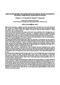
Fig. (11) Standard deviation and mean for the KC and Normal cases . DOI: 10.9790/3008-1206065058
www.iosrjournals.org
57 | Page
Support Vector Machine for Keratoconus Detection by Using Topographic Maps with the Help of .. From table( 4,5) and figure(11).There are small differences in the mean for the top and bottom halves for the normal and KC cases, but there is big difference for the mean between the angle of skewing for the normal and the KC cases, also there is big difference between the mean for the subjective axis between the normal cases and the KC cases. The angle of skewing for the KC is greater than that for the normal one, the standard deviation is higher for the KC so is the subjective axis. the mean value for the top half area for the KC is higher than that for the normal case, while the standard deviation for the top half for KC is smaller than that for the normal case, the area of the bottom half for the normal case is higher than that for the KC, while the standard deviation is higher than that for the normal case.
V. Conclusion 1.
The area of the top half for the circle with diameter of 6mm for the eye in the Keratoconus case is higher than that for the normal case for the mean value, while for the standard devation value is smaller than that for the normal case. The Keratoconus case has lower area of the bottom half value than that for the normal case for the mean value, while for the standard deviation value area of the bottom half in the Keratoconus case is higher than that for the normal case. The confusion matrix shows that the SVM classifier has predicted the KC cornea with an excellent accuracy of 100%, whereas there is an accuracy of 83.3% for the normal cornea but the SVM classifier has wrongly predicted the normal cornea as KC cornea with an accuracy of 16.7%. To say that the case is normal or has a Keratoconus the (12) features which are calculated in table(1) must be obtained and satisfy for all (10) cases to judge that the case is normal or it is in risk case.
2.
3.
4.
Reference [1]. [2]. [3]. [4]. [5]. [6]. [7]. [8]. [9].
[10]. [11]. [12]. [13].
[14]. [15]. [16]. [17]. [18].
R. A. U, J. S. Suri, and E. Y. K. Ng, Disease, Facts About the Cornea and Corneal, Norwood, United States: Artech House Publishers, 2016. E. Addo, O. A. Bamiro, and R. Siwale, “Anatomy of the Eye and Common Diseases Affecting the Eye,” in Ocular Drug Delivery: Advances, Challenges and Applications, USA: Springer International Publishing AG, 2016, pp. 11–26. P. A. Accardo and S. Pensiero, “Neural network-based system for early keratoconus detection from corneal topography,” J. Biomed. Inform., vol. 35, pp. 151–159, 2003. M. K. Smolek and S. D. Klyce, “Current Keratoconus Detection Methods Compared With a Neural Network Approach,” Ophthalmol. Vis. Sci., vol. 38, no. 11, pp. 2290–2299, 1997. R. Jain and S. Grewal, “Pentacam : Principle and Clinical Applications,” J. Curr. Glaucoma Pract., vol. 3, no. 2, pp. 20–32, 2009. F. Toutounchian, J. Shanbehzadeh, M. Khanlari, and A. R. Stage, “Detection of Keratoconus and Suspect Keratoconus by Machine Vision,” The International MultiConference of Engineers and Computre Scientist, 2012, vol. I, pp. 14–16. D. Cheboli and B. Ravindran, “Detection of Keratoconus by Semi-Supervised Learning,” in Work- shop on Machine Learning for Health-Care Applications, 2008. M. B. Souza, F. W. Medeiros, D. B. Souza, R. Garcia, and M. R. Alves, “Evaluation of machine learning classifiers in keratoconus detection from orbscan II examinations,” Clin. Sci., vol. 65, no. 12, pp. 1223–1228, 2010. S.N. Mazhir, A. H. Ali, N. K. Abdalameer,and F. W. Hadi, "Studying the effect of Cold Plasma on the Blood Using Digital Image Processing and Images Texture analysis," International conference on Signal Processing, Communication, Power and Embedded System (SCOPES), IEEE Xplore Digital Library,2016,904-914. S. N. Mazhir, F. W. Hadi, A. N. Mazher, L. H. Alobaidy,"Texture Analysis of smear of Leukemia Blood Cells after Exposing to Cold Plasma", Baghdad Science Journal, Vol.14(2), 2017,403-410. George B. Thomas Jr.and Ross L. Finney ,"Calculus and Analytic Geometry"Addison-Wesley Publishing Company; 6th edition (1986). S. O’HARA and B. A. Draper, “Introduction to the bag of features paradigm for image classification and retrieval,” in Colorado State Uniersity , Computer Science Department , Fort CollIins 2011,. July, pp. 1–25. C. Barata, M. Ruela, T. Mendonça, and J. S. Marques, “A Bag-of-Features Approach for the Classification of Melanomas in Dermoscopy Images : The Role of Color and Texture Descriptors,” in Computer Vision Techniques for the Diagnosis of Skin Cancer, Series in BioEngineering, J. Scharcanski and M. E. Celebi, Eds. Berlin: Springer-Verlag Berlin Heidelberg, 2014, pp. 49– 69. H. M. Abduljabar, T. A. H. Naji, and A. J. Hatem, “Satellite Images Unsupervised Classification Using Two Methods Fast Otsu and K-means Abstract : Introduction : Materails and Methods : Method : Results and Discussions :,” Baghdad Sci. J., vol. 8, no. 2, 2011. Amit David, Boaz Lerner, "Support Vector Machine-Based Image Classification for Genetic Syndrome Diagnosis", Pattern Recognition Letters 26,2005, 1029–1038. A. Ghaaliq, L. Mb, C. Frca, A. Mccluskey, and M. B. Chb, “Clinical tests : sensitivity and specificity,” Contin. Educ. Anaesthesia, Crit. Care Pain, vol. 8, no. 6, pp. 221–223, 2008. T. Mean and T. S. Deviation, “Calculating the Mean and Standard Deviation,” 2017. D.Moore,. G. McCabe, Introduction to the Practice of Statistics, 3th Edition. Freeman, 1998.
Alyaa H.Ali "Support Vector Machine for Keratoconus Detection by Using Topographic Maps with the Help of Image Processing Techniques." IOSR Journal of Pharmacy and Biological Sciences (IOSR-JPBS) 12.6 (2017): 50-58. DOI: 10.9790/3008-1206065058
www.iosrjournals.org
58 | Page